Bookkeeping & Excel - Analysis columns conversion for Pivot Table reporting


40 years working with one to two person businesses . In EE my focus is Excel bookkeeping & accounts & banking. (Not VBA)
Published:
Browse All Articles > Bookkeeping & Excel - Analysis columns conversion for Pivot Table reporting
By an accountant
This will work for anyone anywhere,
Assumptions
That you have a traditional extended analysis spreadsheet you want to convert - I.T. people might better associate with the word "normalise" (NOT as in database normalisation) where data needs to be made database query friendly (and of course being MS Query or Pivot Table friendly can themselves be different things).
So here we go.
First a look at the overview, always acquire an idea of what we are dealing with:
![Traditional Bookkeeping Spreadsheet]()
Readers may like to double click the image above so it opens in a separate browser window and will be much larger: it is a screen shot of a 30" screen. I suggest using full width of your screen and having this article separate for viewing of both.
It does not matter if the image does not identify the details for you; what it does is show us the shape of the monster. We can see:
STEP ONE
Let's see how long this takes me, bearing in mind I am writing this article at the same time. Bear in mind that what you are about to see/do will be the same pretty much regardless of the amount of data / number of rows.
Also note that we are not using any spreadsheet clever tricks, this is merely an accountant (me) talking through a bookkeeping process using typical Excel methods, something you won't really see much of anywhere.
I have prepared a video of this process, here
http://www.youtube.com/watch?v=u4qBAvYTPtg
Steps are:
As I mentioned at the beginning of this step one, remember that this will work for any amount of data, there maybe thousands of entries and the same methods apply.
STEP TWO - NARRATIVE
Now then, this is the tricky bit. We need a way to convert the headings across the top, into labels against each transaction.
We can see that each amount is entered so many columns across.
We can see that each heading is entered so many columns across.
We just need to be able to use the number of columns across for each amount, to tell us which heading to pick up according to the correct heading's location.
Excel's MATCH formula can be persuaded into doing this, because each row has only ONE entry in it so MATCH cannot get it wrong if told to give us the answer regardless of the amount - so we tell MATCH to give us the position of the first entry it finds less than 999 (our numbers are in the hundreds so 999 is infinity as far as our numbers are concerned, add 9s to suit your purpose, this number MUST exceed your largest amount.) MATCH has various requirements, but our need here means pretty much none of them need concern us.
So our logic is: "MATCH, please tell us the number of columns across for the single amount entered in each row, regardless of what that amount may be".
Excel's INDEX formula will then use MATCH's result to read the column number Heading x columns across for each amount.
Copy that down and all the headings magically appear for us, each against its related transaction.
Convert all results to values and we have completed the conversion.
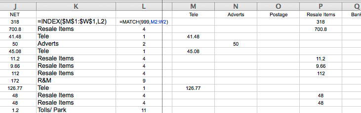
STEP TWO - FORMULAE
Where we have one plus or minus amount entered somewhere in Row 2 in columns M to W and we want to know how many columns it is into that range of columns M to W.
Insert a new column L (i.e. OUTSIDE the range to be looked at)
=MATCH(999,M2:W2) (display the number of columns across that holds any number < 999)
Copy this down in a column inserted for the purpose, say Column L, against every transaction to be "converted".
Now insert another column next to this one, say Column K, with this in Row 2 i.e. in K2,
=INDEX($M$1:$W$1,L2)
where the related headings are in M1 to L1 and the MATCH result is in L2.
What that is doing is reading off the heading associated with the position number shown in L2.
The real trick in all of this is even knowing that this can be done - that is the hard part. The rest is just a case of asking the right questions.
Here it is showing the formulae in place:
![Match and Index capture headings]()
Then
and proceed with Pivot Table reporting, including reproduction of all the extended analysis columns just to prove it can be done.
Without this process it can take hours to do this conversion, it may even not be practicable, involving sorting by each column and copying headings. A small example as in this article is one thing, but as the transaction volumes grow, so does the time and risk of error.
One thing: make SURE there is no more than one item in each extended analysis column. Sometimes they (users) split amounts across columns. The cure for that is replicate the transaction over multiple rows; it's a fix/workaround and rare, so watch for it. It may be wise before starting to insert a column and use COUNT to check ALL the extended analyses do contain only one entry and if more, split them up into one per row. This is the only compromise and in small businesses is not frequent.
Suggestions for improvement are welcome.
Good luck!
Anthony
1. Why this subject?
Because today I was speaking with someone who described to me their old fashioned cross cast analysis bookkeeping spreadsheet. That means lots of headings and each expense "extended" into its appropriate column. I wrote an earlier article about how to do this with modern Excel tools; so that's why this subject.2. Who is this for?
This is for people who have created bookkeeping spreadsheets as I describe above and now who would like to be able to transition from the old way to the new. Doing it manually is really quite laborious. Most are not VBA skilled (including me) so that leaves using any available tricks to be able to ring the changes and minimise the data re-entry, or indeed avoid it altogether.3. Where? Country:
This will work for anyone anywhere,
4. What you need to know:
You need to be reasonably proficient in manipulating your spreadsheet, how to enter formulae, copy and paste them, and "paste special values" to get rid of transitional formulae when we are finished.MOTIVATION
To save myself some time and offer the same ideas to users that I use for myself. Not least to provide myself with a memory aide in the form of an article I can refer to for myself, and if others can benefit from it so much the better. Indeed I will gladly edit this as an ongoing work in progress if and as further techniques become apparent and are found useful.INTRODUCTION OF CONCEPTS & ASSUMPTIONS
Concepts
We do NOT use extended analysis across columns such as “Motor”, “Stationery” etc, because such reports can be produced as a (pivot table or others) report after the data entry work is complete, if still required. In words of one syllable this means you are not allowed more columns across - on pain of a serious increase in professional fees if you do, because it wastes a lot of time and causes grave misunderstandings.
Given the above point this is about converting extended analysis spreadsheets (like the old 13 column analysis of old) into what amount to database like spreadsheets, so we can use those reporting techniques, such as pivot tables.
Assumptions
That you have a traditional extended analysis spreadsheet you want to convert - I.T. people might better associate with the word "normalise" (NOT as in database normalisation) where data needs to be made database query friendly (and of course being MS Query or Pivot Table friendly can themselves be different things).
So here we go.
First a look at the overview, always acquire an idea of what we are dealing with:
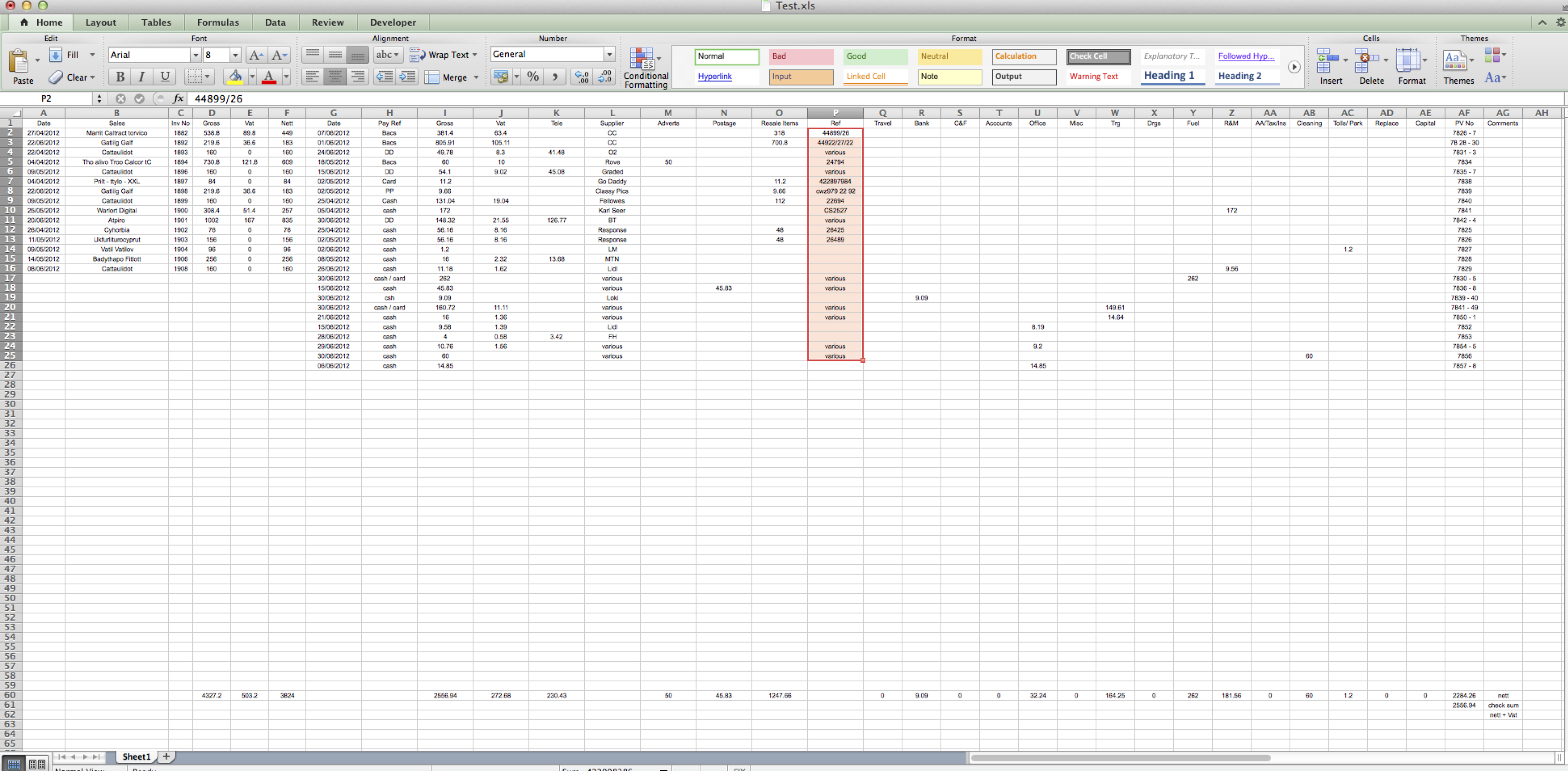
Readers may like to double click the image above so it opens in a separate browser window and will be much larger: it is a screen shot of a 30" screen. I suggest using full width of your screen and having this article separate for viewing of both.
It does not matter if the image does not identify the details for you; what it does is show us the shape of the monster. We can see:
there are a lot of blank rows we can delete immediately.
there are unused columns which we can delete, after keeping a note of them elsewhere, because these represent the business user's desired analyses, which at this point in the proceedings we are not here to argue with, we accept and move on.
there are columns within the area containing the extended analysis that have nothing to do with analysis, such as column P. This is a reference column that belongs on the left.
likewise column AF and column AG. We can see why they are where they are, but for our purposes we will move them.
there is a Gross column and a VAT (sales tax) column, but no Net column. Reason is that the Net is the amount extended across.
this is a very traditional layout in that it even reproduces the left and right pages of the original pre-computer era books of account, Sales/Receipts (debits) on the left and Purchases/Expenditure (Credits) on the right. NOT to be confused with looking at bank statements which are reversed.
all entries are positive. So receipts and expenditure are NOT shown one as positive and the other as negative. Not necessary as laid out, but where we are going they need to be differentiated so us humans can remain comfortable.
there is a row of totals, we need to keep a copy of these so we can check out final results continue to agree, or that we can explain why they do not, which is always errors in the traditional data input.
STEP ONE
Let's see how long this takes me, bearing in mind I am writing this article at the same time. Bear in mind that what you are about to see/do will be the same pretty much regardless of the amount of data / number of rows.
Also note that we are not using any spreadsheet clever tricks, this is merely an accountant (me) talking through a bookkeeping process using typical Excel methods, something you won't really see much of anywhere.
I have prepared a video of this process, here
http://www.youtube.com/wat
Steps are:
transfer totals and column headings to sheet2 for future use.
delete all the blank rows including the totals
cut and paste (move) the sales/receipts columns to the space beneath the purchases/expenditure columns
move the supplier names to the left of the Gross column
move invoice numbers into the pay ref column
(apologies for the noises on the mic at this point in the video, it does stop.)
convert the sales figures to negatives.
move all the extended analysis one column right to make space for the Net column.
enter the net column formula and copy down
move the ref and PV number columns to join the narrative columns
delete the unused extended analysis columns
insert new columns A and B and enter an index column and a source column showing which book of account each transaction is from.
As I mentioned at the beginning of this step one, remember that this will work for any amount of data, there maybe thousands of entries and the same methods apply.
STEP TWO - NARRATIVE
Now then, this is the tricky bit. We need a way to convert the headings across the top, into labels against each transaction.
We can see that each amount is entered so many columns across.
We can see that each heading is entered so many columns across.
We just need to be able to use the number of columns across for each amount, to tell us which heading to pick up according to the correct heading's location.
Excel's MATCH formula can be persuaded into doing this, because each row has only ONE entry in it so MATCH cannot get it wrong if told to give us the answer regardless of the amount - so we tell MATCH to give us the position of the first entry it finds less than 999 (our numbers are in the hundreds so 999 is infinity as far as our numbers are concerned, add 9s to suit your purpose, this number MUST exceed your largest amount.) MATCH has various requirements, but our need here means pretty much none of them need concern us.
So our logic is: "MATCH, please tell us the number of columns across for the single amount entered in each row, regardless of what that amount may be".
Excel's INDEX formula will then use MATCH's result to read the column number Heading x columns across for each amount.
Copy that down and all the headings magically appear for us, each against its related transaction.
Convert all results to values and we have completed the conversion.
STEP TWO - FORMULAE
Where we have one plus or minus amount entered somewhere in Row 2 in columns M to W and we want to know how many columns it is into that range of columns M to W.
Insert a new column L (i.e. OUTSIDE the range to be looked at)
=MATCH(999,M2:W2) (display the number of columns across that holds any number < 999)
Copy this down in a column inserted for the purpose, say Column L, against every transaction to be "converted".
Now insert another column next to this one, say Column K, with this in Row 2 i.e. in K2,
=INDEX($M$1:$W$1,L2)
where the related headings are in M1 to L1 and the MATCH result is in L2.
What that is doing is reading off the heading associated with the position number shown in L2.
The real trick in all of this is even knowing that this can be done - that is the hard part. The rest is just a case of asking the right questions.
Here it is showing the formulae in place:
Then
convert column L to values.
Add a column heading of say "CODE".
delete all analysis columns
and proceed with Pivot Table reporting, including reproduction of all the extended analysis columns just to prove it can be done.
Without this process it can take hours to do this conversion, it may even not be practicable, involving sorting by each column and copying headings. A small example as in this article is one thing, but as the transaction volumes grow, so does the time and risk of error.
One thing: make SURE there is no more than one item in each extended analysis column. Sometimes they (users) split amounts across columns. The cure for that is replicate the transaction over multiple rows; it's a fix/workaround and rare, so watch for it. It may be wise before starting to insert a column and use COUNT to check ALL the extended analyses do contain only one entry and if more, split them up into one per row. This is the only compromise and in small businesses is not frequent.
Suggestions for improvement are welcome.
Good luck!
Anthony
40 years working with one to two person businesses . In EE my focus is Excel bookkeeping & accounts & banking. (Not VBA)
Have a question about something in this article? You can receive help directly from the article author. Sign up for a free trial to get started.
Comments (0)