

Browse All Articles > Cascading Validation Lists
Here’s the scenario: on our worksheet, we want to choose a Country and the corresponding City. We want to limit the countries available to the user as well as the cities that they can choose. For start, we want to choose the country and on the second cell we can only put cities that correspond to that country. It makes sense, right?
So, let’s start we our simple example on how we can make cascading (or dependent) Validation Lists. In cell A2 we want to put the country and on cell B2 we want to put the city, like this example:
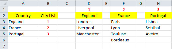
![CVL1]() To start, we have to build our “database”. On a second sheet, I’ve made a list of countries that I want to have available for the user to choose on my validation list and I put an index number that will correspond to the right cities list. So, for instance, for France, I used the index 2 that will be corresponding to the cities list 2. You will see later how this index number will be used.
To start, we have to build our “database”. On a second sheet, I’ve made a list of countries that I want to have available for the user to choose on my validation list and I put an index number that will correspond to the right cities list. So, for instance, for France, I used the index 2 that will be corresponding to the cities list 2. You will see later how this index number will be used.
![CVL2]() Now, if you’re using Excel 2010, you can have the “source” lists on a separated sheet but if you’re using Excel 2003 for instance, you can only have the values on a second sheet if you use named ranges. We will use the name ranges so that this cascading validation lists work on both versions.
Now, if you’re using Excel 2010, you can have the “source” lists on a separated sheet but if you’re using Excel 2003 for instance, you can only have the values on a second sheet if you use named ranges. We will use the name ranges so that this cascading validation lists work on both versions.
So, the next step is to create the named ranges for our lists. On your Formulas tab, we have the Name Manager button. When you click it, it will open the Name Manager dialog box.
![CVL3]()
Click on the New button to add a new named range and it will open the New Name dialog box.
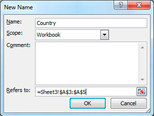
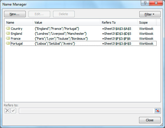
![CVL4]() On the Name field you can put, for instance, “Country” for our first named range and on the “Refers to” field we will select, in this case, =Sheet3!$A$3:$A$5 to get the list of countries. Click OK to finish. Then we need to create the named ranges for the rest of the lists. Click again on the New button on the Name Manager dialog box and repeat the process to create three more named ranges: England, France and Portugal, selecting for the “Refers to” field the corresponding range of cities names. This will leaves with 4 named ranges, like this:
On the Name field you can put, for instance, “Country” for our first named range and on the “Refers to” field we will select, in this case, =Sheet3!$A$3:$A$5 to get the list of countries. Click OK to finish. Then we need to create the named ranges for the rest of the lists. Click again on the New button on the Name Manager dialog box and repeat the process to create three more named ranges: England, France and Portugal, selecting for the “Refers to” field the corresponding range of cities names. This will leaves with 4 named ranges, like this:
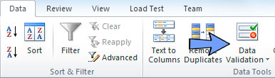
![CVL5]() Now we can build our validations lists on our original sheet where we want to select the data from our “database”. With cell B1 selected (where we want to select our country), go to the Data tab and click on Data Validation and choose Data Validation.
Now we can build our validations lists on our original sheet where we want to select the data from our “database”. With cell B1 selected (where we want to select our country), go to the Data tab and click on Data Validation and choose Data Validation.
![CVL6]() This will open the Data Validation dialog box.
This will open the Data Validation dialog box.
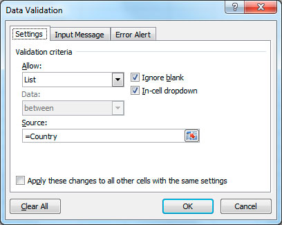
![CVL7]() Now we want to use a list of options for the user to select so go ahead and on “Allow” change the value to “List”. This will open the Source field that is where we will put our Country named range. So put =Country and click OK. Now we want to make the second Validation List for the user to choose the city. Select, in this case, cell B2 that is where we will put this second validation list. Now comes the trick. We need to check the value of the country cell (cell B1) to get the index of the corresponding value on our “database”. If the user selected Portugal we need to get the index “3” that will tell us to get the list of cities that correspond to Portugal. For that we will make a VLOOKUP of the value in cell B1 in the Countries table. After we get the index value, we will “choose” the list to use for the Source of our second validation list. To make this we will use this formula:
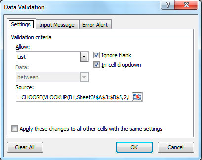
Now we want to use a list of options for the user to select so go ahead and on “Allow” change the value to “List”. This will open the Source field that is where we will put our Country named range. So put =Country and click OK. Now we want to make the second Validation List for the user to choose the city. Select, in this case, cell B2 that is where we will put this second validation list. Now comes the trick. We need to check the value of the country cell (cell B1) to get the index of the corresponding value on our “database”. If the user selected Portugal we need to get the index “3” that will tell us to get the list of cities that correspond to Portugal. For that we will make a VLOOKUP of the value in cell B1 in the Countries table. After we get the index value, we will “choose” the list to use for the Source of our second validation list. To make this we will use this formula:
=CHOOSE(VLOOKUP(B1,Sheet3!$A$3:$B$5,2,FALSE),England,France,Portugal)
So, what does this formula do? It will start for looking up the value on cell B1 against the values on our countries table and getting the corresponding index that it will use on the CHOOSE() function to get either the 1st, 2nd or 3rd named range.
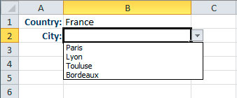
This is how our second validation list will look:
![CVL8]() The result will be two cascading or dependent Validation Lists. If we choose country France, we will have on the cities Validation List the cities from France only.
The result will be two cascading or dependent Validation Lists. If we choose country France, we will have on the cities Validation List the cities from France only.
![CVL9]() This article demonstrates how you can make basic cascading Validation Lists to use on your sheets. You can take this example and use it on your own real life situations.
This article demonstrates how you can make basic cascading Validation Lists to use on your sheets. You can take this example and use it on your own real life situations.
So, let’s start we our simple example on how we can make cascading (or dependent) Validation Lists. In cell A2 we want to put the country and on cell B2 we want to put the city, like this example:
 To start, we have to build our “database”. On a second sheet, I’ve made a list of countries that I want to have available for the user to choose on my validation list and I put an index number that will correspond to the right cities list. So, for instance, for France, I used the index 2 that will be corresponding to the cities list 2. You will see later how this index number will be used.
 Now, if you’re using Excel 2010, you can have the “source” lists on a separated sheet but if you’re using Excel 2003 for instance, you can only have the values on a second sheet if you use named ranges. We will use the name ranges so that this cascading validation lists work on both versions.
So, the next step is to create the named ranges for our lists. On your Formulas tab, we have the Name Manager button. When you click it, it will open the Name Manager dialog box.

Click on the New button to add a new named range and it will open the New Name dialog box.
 On the Name field you can put, for instance, “Country” for our first named range and on the “Refers to” field we will select, in this case, =Sheet3!$A$3:$A$5 to get the list of countries. Click OK to finish. Then we need to create the named ranges for the rest of the lists. Click again on the New button on the Name Manager dialog box and repeat the process to create three more named ranges: England, France and Portugal, selecting for the “Refers to” field the corresponding range of cities names. This will leaves with 4 named ranges, like this:
 Now we can build our validations lists on our original sheet where we want to select the data from our “database”. With cell B1 selected (where we want to select our country), go to the Data tab and click on Data Validation and choose Data Validation.
 This will open the Data Validation dialog box.
 Now we want to use a list of options for the user to select so go ahead and on “Allow” change the value to “List”. This will open the Source field that is where we will put our Country named range. So put =Country and click OK. Now we want to make the second Validation List for the user to choose the city. Select, in this case, cell B2 that is where we will put this second validation list. Now comes the trick. We need to check the value of the country cell (cell B1) to get the index of the corresponding value on our “database”. If the user selected Portugal we need to get the index “3” that will tell us to get the list of cities that correspond to Portugal. For that we will make a VLOOKUP of the value in cell B1 in the Countries table. After we get the index value, we will “choose” the list to use for the Source of our second validation list. To make this we will use this formula:
=CHOOSE(VLOOKUP(B1,Sheet3!
So, what does this formula do? It will start for looking up the value on cell B1 against the values on our countries table and getting the corresponding index that it will use on the CHOOSE() function to get either the 1st, 2nd or 3rd named range.
This is how our second validation list will look:
 The result will be two cascading or dependent Validation Lists. If we choose country France, we will have on the cities Validation List the cities from France only.
 This article demonstrates how you can make basic cascading Validation Lists to use on your sheets. You can take this example and use it on your own real life situations.
Have a question about something in this article? You can receive help directly from the article author. Sign up for a free trial to get started.
Comments (4)
Commented:
Dave
Commented:
Commented:
could you please provide the example code for Index/Match
Commented:
=INDIRECT($B$1)
Book1.xlsx