Help with Excel Spreadsheet and formulas
I am looking for a solution to a problem I am having with this document.
Explanation of the document-
The document has 4 pages –
MRPExport – This is where the purchasing recommendations are pasted
MRP Recommendations with lead – (Main Sheet) - This combines information form MRPExport and Items Sheet and runs some Calculations
Items – This is a list of items from the system which contains some extra information than MRPExport
Exchange Rates – this is used to convert all Currencies into GBP
As you can see I have two totals in AQ2 and AR2, the problem is that these totals are not correct, AQ2 is calculated by - Actual Quantity Column * Cost Column. AR2 is calculated by – Adjusted Quantity Column * Cost Column
These totals are designed to show the total costs of all the purchase orders recommended by the system.
The Problem –
As well as recommending new purchase order (new P/O), this document also recommends to cancel Purchase orders (Cancel P/O) unfortunately the system does not record the prices for the cancellation recommendations only the ‘new P/O recommendations’. As a result the total costs are not accurate.
NOTE - When there is a ‘Cancel P/O’ There is not always a ‘new P/O’ Recommendation.
Solution –
I need the cost column to display the cost of the item in minus figures for lines that contain the word Cancel in the Message column, AND have the same item on a PO Recommendation so that they will be subtracted from the total.
Summary –
The Formula needs to do this -
Put a Minus figure of the Cost of the Product Code in column ‘Cost’ Under these conditions –
There is a Cancel Recommendation in the Message Column AND a New P/O Recommendation in the message column for the same Product Code. If there is no New P/O recommendation it should put a 0 in the Cost Column. It should also show a positive Cost for all other items.
Calculations-Document.xlsx
ASKER
Many thanks. Which column does this need to go in?
Starting in O2 of "MRP Recommends with Lead" sheet, copied down
ASKER
This doesn't work! I get an error message - please see attached
Error.docx
Error.docx
ASKER
This doesn't work! I get an error message - please see attached
All you need to is hit Enter. You probably didn't copy all the brackets in my formula so Excel is letting you know...
ASKER
Yes I had missed off a bracket at the end when copying. I have corrected this so I no longer get a warning.
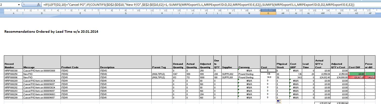
However I still don't see any change. The lines that have a 'Cancel' recommendation (and have a New P/O recommendation) should display a Minus figure of the cost, but they still show 0 as before. see image below after your formula has been entered.
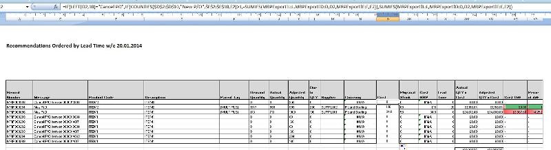
However I still don't see any change. The lines that have a 'Cancel' recommendation (and have a New P/O recommendation) should display a Minus figure of the cost, but they still show 0 as before. see image below after your formula has been entered.
Which ones?
Item 1 is the only duplicated item and the corresponding cost in columm L on the other sheet is 0.
Can you please indicate the expected results for this sample along with explanation of where it came from and why.
Item 1 is the only duplicated item and the corresponding cost in columm L on the other sheet is 0.
Can you please indicate the expected results for this sample along with explanation of where it came from and why.
ASKER
OK Let me try to explain it more clearly, I need the totals columns AN and AO to display positive costs for all New P/O Lines, (it already does this)
AND
Negative Costs for all Cancel P/O Lines (It currently does not do this)
The Cancel Lines do not show a cost on the MRPexport page, so they will need to draw the cost from the same cell that the new P/O gets the cost from
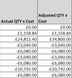
Does that make sense? Sorry it is hard to explain. I want Column AN and AO to look like this -
AND
Negative Costs for all Cancel P/O Lines (It currently does not do this)
The Cancel Lines do not show a cost on the MRPexport page, so they will need to draw the cost from the same cell that the new P/O gets the cost from
Does that make sense? Sorry it is hard to explain. I want Column AN and AO to look like this -
ASKER CERTIFIED SOLUTION
membership
This solution is only available to members.
To access this solution, you must be a member of Experts Exchange.
ASKER
I have managed to get these columns to display minus figures on Cancel lines, but it does it for all lines that have Cancel.
I only want it to show a Minus when there is a New P/O Line for the same item.
Attached is the file as it is now.
Calculations-Document---Bens-edi.xlsx
I only want it to show a Minus when there is a New P/O Line for the same item.
Attached is the file as it is now.
Calculations-Document---Bens-edi.xlsx
Try, in AM2:
=IF(LEFT(MRPExport!D2,6)="
copied down.
=IF(LEFT(MRPExport!D2,6)="
copied down.
ASKER
Thanks a lot, I assume you meant AN2 not AM2...
This still wasn't quite Right as it was returning a Positive value of the Cost for items that were only showing a cancel and not both a cancel and New PO, but I adjusted it to this -
=IF(LEFT(MRPExport!D10,6)=
And now it works just right! :) Thanskyou so much for your help and your patience with me!
Kind Regards, Ben.
Ok. You're welcome. Glad you got to the desired end result finally.
ASKER
After reviewing this it is still not correct.
The problem now is that the minus figures for Item1 are greater than the new P/O cost of Item1 so the total shows a minus figure.
What I actually need it to is the following -
If there is a Cancel P/O and New P/O for any item, add up the total cost of all the Cancel P/O for that item, and minus that from the Cost of the New P/O THEN If the answer is less than zero show Zero in column AM, if it is more than zero, show that cost in AM
What happens to the New P/O value for that item?
ASKER
The total value (Cost*actual quantity) for that item, will be reduced by deducting the total of all the Cancel P/O costs*actual Quantities for that item.
So in the case of Item1
if it recommends 1000pcs on the new P/O line, but the cancellations add up to 900, it will only show a cost of 100*34.8 in the Column AM
So in the case of Item1
if it recommends 1000pcs on the new P/O line, but the cancellations add up to 900, it will only show a cost of 100*34.8 in the Column AM
Let's give this one a try:
=IF(D2="New P/O",ABS(SUMPRODUCT(--($D$2:$D$10="New P/O"),--($E$2:$E$10=E2),$J$2:$J$10,$P$2:$P$10)-SUMPRODUCT(--(LEFT($D$2:$D$10,6)="Cancel"),--($E$2:$E$10=E2),$J$2:$J$10,$P$2:$P$10)),IF(SUMPRODUCT(--($D$2:$D$10="New P/O"),--($E$2:$E$10=E2),$J$2:$J$10,$P$2:$P$10)-SUMPRODUCT(--(LEFT($D$2:$D$10,6)="Cancel"),--($E$2:$E$10=E2),$J$2:$J$10,$P$2:$P$10)<0,0,J2*P2))ASKER
Sorry but I pasted this in AM2 and copied down.
I got a huge number - 45824900
I have a P/o recommendation for 1000pcs at 34.8 = £34800.00
I have cancellations for ITEM1 that total = £32155.20
So I am expecting AM2 to show £34800.00 - £32155.20 = £2644.80
I got a huge number - 45824900
I have a P/o recommendation for 1000pcs at 34.8 = £34800.00
I have cancellations for ITEM1 that total = £32155.20
So I am expecting AM2 to show £34800.00 - £32155.20 = £2644.80
In the sample workbook you provided, I got close to your number.. (I don't know your exact numbers for the cancelled pos so I adusted the numbers in column J to get close to you) but the result indicates the numbers work....
Calculations-Document---Bens-edi.xlsx
Calculations-Document---Bens-edi.xlsx
ASKER
Thanks, Sorry, don't know what I had done on the sheet I was using!
This is looking good, the reason it is close and not Exactly the same number, is because the Cost values show 38 instead of 34.8.
This is taking the cost from the supplier on the items sheet.
If it took it form the MRPExport sheet instead, It would work perfectly.
Can you help me to figure this last bit out please?
From column L? I see 0's for those canceled PO's, is that what should go in the Cost column of MRP Recommends with Lead sheet?
ASKER
It depends how your calculation works on AN?
As long as it does the deduction of the cancel Orders from the new PO correctly. and as you say it is close but not quite right. I think it must be that these show 38 rather 34.8??
As long as it does the deduction of the cancel Orders from the new PO correctly. and as you say it is close but not quite right. I think it must be that these show 38 rather 34.8??
ASKER
it would need to read from the new P/O Item1 cost if it did need to display it.
Try:
=SUMIFS(MRPExport!L:L,MRPE
=SUMIFS(MRPExport!L:L,MRPE
ASKER
Hi this is good, the attached is working right except for one thing.
if the Actual Quantity for a new P/O item is lower than the total quantity of all the Cancellations added together, the new P/O Line should return a zero in the AL column.
At the moment it is still showing the actual QTY*cost.
Calculations-Document---Bens-edi.xlsx
Thanks, Ben.
if the Actual Quantity for a new P/O item is lower than the total quantity of all the Cancellations added together, the new P/O Line should return a zero in the AL column.
At the moment it is still showing the actual QTY*cost.
Calculations-Document---Bens-edi.xlsx
Thanks, Ben.
.... becoming confusing ...
try:
copied down
try:
=IF(AND(D2="New P/O",(SUMPRODUCT(--($D$2:$D$10="New P/O"),--($E$2:$E$10=E2),$I$2:$I$10,$N$2:$N$10)-SUMPRODUCT(--(LEFT($D$2:$D$10,6)="Cancel"),--($E$2:$E$10=E2),$I$2:$I$10,$N$2:$N$10))<0),0,IF(SUMPRODUCT(--($D$2:$D$10="New P/O"),--($E$2:$E$10=E2),$I$2:$I$10,$N$2:$N$10)-SUMPRODUCT(--(LEFT($D$2:$D$10,6)="Cancel"),--($E$2:$E$10=E2),$I$2:$I$10,$N$2:$N$10)<0,0,I2*N2))copied down
ASKER
Yes it is a bit confusing, it is hard to explain what is needed.
This Formula does put a Zero if the Actual Quatity is less that the Canceled total qty as I asked.
But it has now stopped working the other way around.
It needs to do both, when the Actual QTY is less than Combined Cancel lines it needs to show Zero. (as it does now with your new formula)
When it is Higher it needs to show the difference (as the previous formula did)
Does that make sense?
Let's see if this is the winning formula:
=IF(AND(D2="New P/O",(SUMPRODUCT(--($D$2:$D$10="New P/O"),--($E$2:$E$10=E2),$I$2:$I$10,$N$2:$N$10)-SUMPRODUCT(--(LEFT($D$2:$D$10,6)="Cancel"),--($E$2:$E$10=E2),$I$2:$I$10,$N$2:$N$10))<0),0,IF(D2="New P/O",ABS(SUMPRODUCT(--($D$2:$D$10="New P/O"),--($E$2:$E$10=E2),$I$2:$I$10,$N$2:$N$10)-SUMPRODUCT(--(LEFT($D$2:$D$10,6)="Cancel"),--($E$2:$E$10=E2),$I$2:$I$10,$N$2:$N$10)),IF(SUMPRODUCT(--($D$2:$D$10="New P/O"),--($E$2:$E$10=E2),$I$2:$I$10,$N$2:$N$10)-SUMPRODUCT(--(LEFT($D$2:$D$10,6)="Cancel"),--($E$2:$E$10=E2),$I$2:$I$10,$N$2:$N$10)<0,0,I2*N2)))ASKER
It Works!!! :)
I have a bigger sheet that I need to add these formula's to to make sure they still work.
IF I get further problems I will let you know once I have checked it through.
Thanks again.
I have a bigger sheet that I need to add these formula's to to make sure they still work.
IF I get further problems I will let you know once I have checked it through.
Thanks again.
Great. Let me know the outcome.
ASKER
Hi There,
Thanks for your help so far with this, I can report that it is working correctly.
There is one more thing I need your help with.
I need this formula to work in the column next to the one it currently does as well, effectively I need to sort of shift this formula so that it works in the "Adjusted Qty x Cost" column as well.
It should be the same calculations, but looking at the Adjusted QTY column instead of the Actual Qty Column.
Doing this will allow me to compare these two columns to see the differences in cost. between ordering the Actual Qty we need against the adjusted Qty it suggests to buy.
Thanks.
Would that be?
=IF(AND(D2="New P/O",(SUMPRODUCT(--($D$2:$D$10="New P/O"),--($E$2:$E$10=E2),$J$2:$J$10,$N$2:$N$10)-SUMPRODUCT(--(LEFT($D$2:$D$10,6)="Cancel"),--($E$2:$E$10=E2),$J$2:$J$10,$N$2:$N$10))<0),0,IF(D2="New P/O",ABS(SUMPRODUCT(--($D$2:$D$10="New P/O"),--($E$2:$E$10=E2),$J$2:$J$10,$N$2:$N$10)-SUMPRODUCT(--(LEFT($D$2:$D$10,6)="Cancel"),--($E$2:$E$10=E2),$J$2:$J$10,$N$2:$N$10)),IF(SUMPRODUCT(--($D$2:$D$10="New P/O"),--($E$2:$E$10=E2),$J$2:$J$10,$N$2:$N$10)-SUMPRODUCT(--(LEFT($D$2:$D$10,6)="Cancel"),--($E$2:$E$10=E2),$J$2:$J$10,$N$2:$N$10)<0,0,J2*N2)))ASKER
Yes this seems to work, thanks.
ASKER
Hi there,
I have a further problem with this.
Firstly the current formulas only look at the first 10 lines of the columns, but I need it to look at the entire column as there will be other lines added to this document.
For example - $D$2:$D$10="New P/O" is it as simple as changing it to - D:D="New P/O" ?
Secondly, the lines that have a Cancel need to output a zero in both the "Actual QTYxCost" and "Adjusted QtyxCost" columns, otherwise the totals at the bottom are incorrect as it adds them up.
Can we compare to AM column and say that if AM=0 then return 0, otherwise continue with the calcs?
e.g.
Also, It is not recommended to use whole columns like D:D with SUMPRODUCT because it is not an efficient function and will slow down the processing significantly. Instead use a range that will be large enough that it should never be exceeded, but not excessively large.
You can select the two column and do a FIND/REPLACE (ALT+H). Replace $10 with $1000 or whatever number you choose to be your max range size.
e.g.
=IF(AM2=0,0,IF(AND(D2="New P/O",(SUMPRODUCT(--($D$2:$D$10="New P/O"),--($E$2:$E$10=E2),$J$2:$J$10,$N$2:$N$10)-SUMPRODUCT(--(LEFT($D$2:$D$10,6)="Cancel"),--($E$2:$E$10=E2),$J$2:$J$10,$N$2:$N$10))<0),0,IF(D2="New P/O",ABS(SUMPRODUCT(--($D$2:$D$10="New P/O"),--($E$2:$E$10=E2),$J$2:$J$10,$N$2:$N$10)-SUMPRODUCT(--(LEFT($D$2:$D$10,6)="Cancel"),--($E$2:$E$10=E2),$J$2:$J$10,$N$2:$N$10)),IF(SUMPRODUCT(--($D$2:$D$10="New P/O"),--($E$2:$E$10=E2),$J$2:$J$10,$N$2:$N$10)-SUMPRODUCT(--(LEFT($D$2:$D$10,6)="Cancel"),--($E$2:$E$10=E2),$J$2:$J$10,$N$2:$N$10)<0,0,J2*N2))))Also, It is not recommended to use whole columns like D:D with SUMPRODUCT because it is not an efficient function and will slow down the processing significantly. Instead use a range that will be large enough that it should never be exceeded, but not excessively large.
You can select the two column and do a FIND/REPLACE (ALT+H). Replace $10 with $1000 or whatever number you choose to be your max range size.
ASKER
Hi there,
This formula doesn't seem to work at all, it says it is a circular formula and turns all of them to 0.
Can you tell me which document you are using and which column you are using this formula in? Just so I am sure that its not my fault!?
This formula doesn't seem to work at all, it says it is a circular formula and turns all of them to 0.
Can you tell me which document you are using and which column you are using this formula in? Just so I am sure that its not my fault!?
I used the one that shows up first here:
https://www.experts-exchange.com/questions/28349935/Help-with-Excel-Spreadsheet-and-formulas.html?anchorAnswerId=39835262#a39835262
and the formula is put in AN2, and copied down.
https://www.experts-exchange.com/questions/28349935/Help-with-Excel-Spreadsheet-and-formulas.html?anchorAnswerId=39835262#a39835262
and the formula is put in AN2, and copied down.
Hi Broadcastwarehouse,
Just checking in to see if this question has been resolved.
Just checking in to see if this question has been resolved.
ASKER
Hi Sorry but this doesn't work, AN is the cost difference column, did you mean AM?
I tried AM too just in case, but it gives me a Circular reference warning.
if I OK the warning it just makes them all go to 0.
I tried AM too just in case, but it gives me a Circular reference warning.
if I OK the warning it just makes them all go to 0.
Sorry, it probably the AL column then.... I am getting confused with the number of changes, etc in this long thread.
ASKER
Sorry this doesn't work, it is no good compring it with the AM column, because the AM column also needs to do the same thing -
The lines that have a Cancel need to output a zero in both the "Actual QTYxCost"(AN)and "Adjusted QtyxCost" (AM) columns, otherwise the totals at the bottom are incorrect as it adds them up.
The lines that have a Cancel need to output a zero in both the "Actual QTYxCost"(AN)and "Adjusted QtyxCost" (AM) columns, otherwise the totals at the bottom are incorrect as it adds them up.
I am afraid I don't know what else to offer. After 42 postings in this thread, I think I am totally confused as to what the goal is anymore....
Open in new window
copied down