robmarr700
asked on
full report macro needed
Hi All,
Attached is a worksheet which contains all of my sales orders YTD.
1.Sheet, 'sales order ytd(end of may)' contains all the sales orders year to date. You will notice from row 9921 downwards many of the columns are missing information. This is because these line's are dedicated to products (codes) which haven't received any orders but for product performance reporting it was important they were included in the data.
Sheet two contains;
2. Sheets, January, February, March, April, May is just the same data separated into the separate months.
3. Customer T.O ytd - just shows a running monthly sales total for each customer for each moth of the year with a ytd total in the final collum.
4. Supplier T.O ytd is essentially the same but by supplier rather than customer.
Aim
So I would like to take this one step further. I would like to be able to (on one sheet) view the suppliers turnover for a chosen customer (chosen using a report filter). The results will be separated into columns for the separate months (jan,feb,march,april,may) with the £ Dif and % Dif in between in exactly the same way I have done so on the Supplier/customer T.O ytd sheets.
I would like to do this in reverse also. e.g. view customer turnover via chosen filtered supplier.
* Note this will be a report I would like to update on an ongoing basis so new sales order data will be added for June, July etc.
I have drawn a diagram of what I am trying to achieve (see attached)
Best of luck and any questions please fire away.
Rob
sales-ytd--end-of-may-.xlsx
29.05.14--sales-figures-.xlsx
ASKER
Please find attached diagram.
*Another idea
It would also be great to be able to select a supplier from the list in the left hand column. This supplier would then expand providing the same information but broken down further into the individual product sales for that member from that supplier.
Rob
diagram-EE-page-001.jpg
*Another idea
It would also be great to be able to select a supplier from the list in the left hand column. This supplier would then expand providing the same information but broken down further into the individual product sales for that member from that supplier.
Rob
diagram-EE-page-001.jpg
This is a large project request, Rob and HUGE files. :-) It may take a little time for an Expert to fully analyze and produce a solution for you.
I'll try to take a look at it in more depth later today.
-Glenn
I'll try to take a look at it in more depth later today.
-Glenn
ASKER
Hi Glenn I did think that. I'm not entirely sure why one of the files is so HUGE!
Let me know if you have any questions.
Rob
Let me know if you have any questions.
Rob
File Size: I can answer that. The second file you attached has the last active cell as being Q1035723 on the January sheet and P1035747 on the February sheet - well past your data range and all blank. This takes up a large amount of memory.
I removed the blank columns and rows and am attaching the updated file (no other edits). It's now only 1.8MB (down from 47.9MB). :-)
-Glenn
EE-29.05.14--sales-figures-.xlsx
I removed the blank columns and rows and am attaching the updated file (no other edits). It's now only 1.8MB (down from 47.9MB). :-)
-Glenn
EE-29.05.14--sales-figures-.xlsx
ASKER
Thanks Glenn,
I'm not really sure how to approach this one.
I think the question needs breaking down into more manageable chunks although I wouldn't know where to start as I don't know what's required.
Perhaps you could help me break the project down so I can split it into 3 or four separate questions?
Rob
I'm not really sure how to approach this one.
I think the question needs breaking down into more manageable chunks although I wouldn't know where to start as I don't know what's required.
Perhaps you could help me break the project down so I can split it into 3 or four separate questions?
Rob
Maybe breaking it down will help. I have admit I was overwhelmed reading it through the first time. I did look at the diagrams, but need to just spend about 10 minutes and then make sure I can re-state it.
ASKER
Hi Glenn,
Right, finally I've had a chance to sit down and have a think about this one and how to break it down. I think the best way to explain what I'm trying to do is to provide a practical scenario.
Scenario
Sheet (Supplier t/o ytd) displays the monthly turnover by supplier YTD. By referring to cell O2 I can see that our highest turnover supplier, Mitutoyo, turnover dropped £17,321.53 from April to May. This is important information however I want to look further into the data to understand why the dramatic drop in turnover.
So my next step would be to establish the monthly t/o of the customers that contribute to Mitutoyo's turnover for each month. Ideally I would like to be able to choose Mitutoyo (or any other supplier) from a report filter. This will then bring up the monthly turnover of customer spend for Mitutoyo in exactly the same format as in the (supplier t/o ytd) sheet e.g. (Feb,March, £Dif, %Dif, total etc. SEE DIAGRAM). So at this point I will be able to look at the customer spend for April and May and highlight which customer's are responsible for the drop in Mitutoyo's t/o.
Being able to use a report filter to choose which Supplier I want to display this information for will make things a lot quicker.
So now lets say (for example) I have highlighted the customers responsible for the drop in turnover. I then want to go another step further and establish which product lines are responsible for those particular customers drop in spend. Ideally each customer in the sheet will have a + sign next to it. By clicking on the + it will expand upon the subtotals (product code sales totals) which will then display the same info as before e.g. feb, march, %Dif, £Dif etc.
See new attached diagram. Note I only used Feb and March to demonstrate. The complete table would display all months ytd.
New data would be added monthly.
Origin of data - Sales orders report
I would also like to do this for customers. e.g highlight drop in a customer sales, select that customer from filter, display supplier t/o break down for that customer, expand on product totals.
I hope this makes more sense than before. Let me know your thoughts.
Rob
diagram-2.jpg
ASKER
Sorry Glenn,
I was wondering whether you'd had a chance to see the above?
thanks
Rob
I was wondering whether you'd had a chance to see the above?
thanks
Rob
SOLUTION
membership
This solution is only available to members.
To access this solution, you must be a member of Experts Exchange.
ASKER
Hi Glenn,
This looks fantastic. I will run some tests and will report back on any potential problems/ideas.
Would you be able to add the same sheet but in reverse? e.g. Customer filter>>supplier break down>>product break down.
I see what you mean about the the #NULL error's. Let me know how you get on with that one.
All in all I'm very happy so far. If I could award for than 500 points I certainly would!
Rob
I had a DOH! moment yesterday, figured out how to hide the error, but forgot to post the updated workbook.
BUT, instead of doing that, I'll make this a quick lesson in hiding PivotTable errors. :-)
As a result, you can remove all the conditional formatting rules for this sheet also; they're no longer necessary.
(Menu: Home, Conditional Formatting, Clear Rules, Clear Rules from Entire Sheet)
-Glenn
BUT, instead of doing that, I'll make this a quick lesson in hiding PivotTable errors. :-)
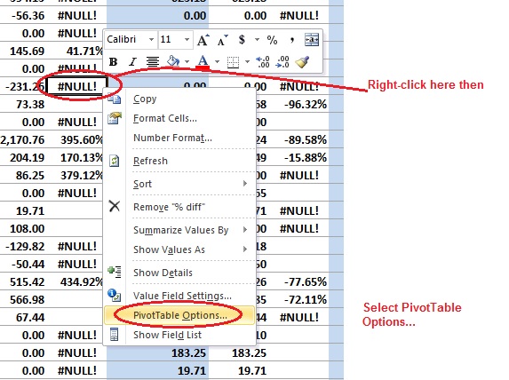
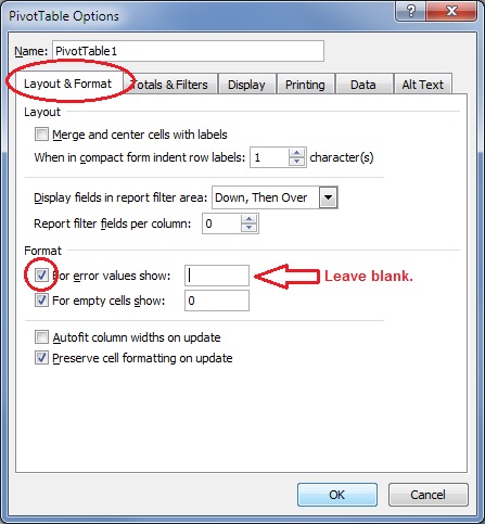
1.
Open the Excel file and view the PivotTable.2.
Right-click on the PivotTable and select "PivotTable Options..."
3.
Select the "Layout & Format" tab then click the checkbox "For error values show:". Leave the box blank.
4.
Click the "OK" button. And they're gone! :-)As a result, you can remove all the conditional formatting rules for this sheet also; they're no longer necessary.
(Menu: Home, Conditional Formatting, Clear Rules, Clear Rules from Entire Sheet)
-Glenn
ASKER
Hi Glenn,
Thats great. Just a couple of questions?
Northern power tools turnover of mitutoyo dropped by 100% from April to May (£14,085.90 to £0.00)
yet the % dif is returning null. This is happening for all customers, do you know why this is?
Also is it not possible to sort the pivot table. For example I would like to list the £Dif list from highest to lowest or vice versa but I am getting an error message?
Thanks
Rob
Hi Rob,
When the values between two adjacent months drops from a positive value to zero, the £ Diff column calculates it as:
[Current Month] - [Previous Month]
Similarly, the % Diff column calculates it as
[Current Month] - [Previous Month]
--------------------------
[Current Month]
If the [Current Month] is zero, you get an error (can't divide by zero); which is what was causing all the #NULL! errors (like the #DIV/0! errors on the "Supplier T.O YTD" sheet".
There is an argument for showing these results as -100%, but that can be misleading since any pair of values that drop to zero would report the same way. Same for zero-to-positive values.
I thought I could sort this, but I'm having the same issue. If I can't find a solution, I'll post another alternative table.
-Glenn
Rob,
I couldn't resolve the issue with the sorting, so I basically started from scratch and re-built the Supplier T.O YTD and Member T.O YTD sheets using SUMIFS to capture the appropriate monthly data. I updated the "Difference" formulas appropriately and now you can sort on any column.
The "Member T.O YTD" sheet also allows you to "drill down" on a specific supplier using value in cell B1). If that cell is left blank, all activity is shown. If you want it to collapse and only show customers with activity for a specific supplier, click on the filter for "Total Sales YTD" and uncheck the box for (Blanks). If you change the supplier value again, you have refresh that filter (cllick on filter arrow and then the OK button again). {This could be automated with a Worksheet_Change event, but I'm holding off on any VBA automation for now}.
You can remove the Pivot Table sheet if you want; it's not being used.
IMPORTANT NOTE: The Member/Customer names needed a lot of cleanup; there were extra spaces and tabs in them. I thought I addressed this in my other solution for you that created the worksheets from the reports, but this needs to be addressed going forward or the formula will not pick up new data.
Speaking of New Data: when you get the June sheet, add it to this workbook, then copy/append all the data to the bottom of the FY2014 sheet (row 15133). You'll need to add "June" to column Q; don't have to add columns R&S.
-Glenn
EE-29.05.14--sales-figures-.xlsx
Hi Rob,
Did you have a chance to review the latest workbook solution? I think it will meet your needs.
-Glenn
Did you have a chance to review the latest workbook solution? I think it will meet your needs.
-Glenn
ASKER
Hi Glenn,
Apologies for the delay in getting back to you.
Thank-you for modifying the member/supplier sheets. I don't know why I didn't use SUMIF's in the first place!
I have noticed that the monthly totals are not the same on the member and supplier t/o sheets. Do you know why this may be?
Also, does this mean it won't be possible to expand on product totals like in the pivot report sheet?
Rob
1) Monthly Total Discrepancies: That is happening because not all Suppliers or Customers are fully listed on their respective sheets. For example, in May you have suppliers with the codes MIR, TRE, 0, and (blank) with Total Sales figures greater than zero. I don't have a quick fix for you here, but have attached a revised version of the workbook so you can see the May issue (I've filtered on the cells with blank or zero as the Supplier code; added new rows for the MIR and TRE codes so you can fill in the appropriate data on the Supplier sheet and Lookup table)
2) No, these sheets will not have "drill down" capability as with a PivotTable.
-Glenn
EE-29.05.14--sales-figures-.xlsx
2) No, these sheets will not have "drill down" capability as with a PivotTable.
-Glenn
EE-29.05.14--sales-figures-.xlsx
ASKER
Hi Glenn,
I see what you mean. I have now amended all of the blank supplier cells so hopefully this should fix things.
You will see the supplier amendments on the attached sheet. I have also added the sheet for June which I have appended as you instructed. Ideally I would like to automate the process of adding the June(and future months) figures to the supplier/member t/o sheets and the drill down pivot table. I'm assuming the drill down pivot will need to be adjusted now the source data has changed?
Also, a heads up.
Tomorrow I will be opening 3 new questions all relating to full parsing of reports. I think they should be fairly straight forward i.e. won't involve much more than cleaning up the data from its txt. file origin.
Master-YTD-1.xlsx
Rob, FYI, I will be unavailable for several days to address any issues or new questions.
-Glenn
Sent from my Windows Phone
-Glenn
Sent from my Windows Phone
ASKER
Hi Glenn,
If you could update me with your'e availability that would be great.
Rob
If you could update me with your'e availability that would be great.
Rob
ASKER
your*
I'll be available after July 17
ASKER
Great, thanks for letting me know
Rob
Rob
ASKER
Hi Glenn,
Attached is the most up to date master sheet. I have cleaned up the customer names so there shouldn't be any duplicates any more. Please refer to my last issue a few comments up. I'd like to continue to use the pivot table as it allows me to drill down on product level sales. I'm desperately trying to update the June figures but have had little success.
I'm happy with the new structure to the supplier/customer t/o sheets.
Let me know if you have any questions
Rob
Master-YTD-3.xlsx
ASKER
Hi Glenn,
Sorry to hassle you but did you get a chance to look at this one?
If you are unable to look at it at the moment I will close the question and open it up as a new question to the rest of the expert community.
Rob
Sorry to hassle you but did you get a chance to look at this one?
If you are unable to look at it at the moment I will close the question and open it up as a new question to the rest of the expert community.
Rob
ASKER CERTIFIED SOLUTION
membership
This solution is only available to members.
To access this solution, you must be a member of Experts Exchange.
Hey Rob,
Just making sure you had a chance to review the updated workbook. I think, if this is acceptible, that this question should be closed and any new issues be address in follow up questions. I do think some change(s) may need to be make in the data preparation tools I developed earlier to handle blank supplier codes and similar.
Regards,
-Glenn
ASKER
Hi Glenn,
Absolutely, great job.
I'm particularly happy that you have corrected the turnover totals so they now match on all sheets.
Assigning 'UNK' to the unknown suppliers was a good idea. There are so few at the moment that it doesn't take long to correct them manually from the information I can see in the descriptions etc.
Great work on this one. Any further issues/queries I have I will post as a new question.
Thanks again
Rob
ASKER
Again impressed with Glenn's ability to understand the needs of a long and complex question; often suggesting new idea's and solutions I hadn't even thought of.
ASKER