asked on

Range of cells equal to a single value in Excel functions

Formula in Excel to display the date for the last occurrence of a value in a table

Hello,

This is a follow-up question to the above thread. The formula given (by Flyster) for the solution was:

=LOOKUP(2,1/(B1:B12=B15),A1:A12)

My question in this thread relates to the denominator of the 2nd term which includes the following:

B1:B12=B15

How can a range of values be equal to a single value?

A range of cells implies multiple values, right? So I understand when a range is part of a function — such as:

a) entering the formula =SUM(B1:B12) in cell B15 or

b) asking if the function of a range is equal to the value in a single cell: =IF(SUM(B1:B12)=B15,1,0)

But what does it mean to put a range of values equal to a single value?

Thanks

Rgonzo1971

Hi,

B1:B12=B15

Returns a list of true or false depending on the values in the range and the value in B15
for example

12
15
14
15
would return
False
True
False
True

Regards

SOLUTION

Rob Henson

membership

This solution is only available to members.

To access this solution, you must be a member of Experts Exchange.

Start Free Trial

ASKER CERTIFIED SOLUTION

barry houdini

membership

This solution is only available to members.

To access this solution, you must be a member of Experts Exchange.

Start Free Trial

WeThotUWasAToad

ASKER

Rob, your statement,

…the function looks at each value in a range as an individual value.

really helps.

Thanks

WeThotUWasAToad

ASKER

You can see this in action using the "Evaluate Formula" Tool

Barry,

Apologies for my belated reply but thanks for mentioning this tool. I've heard about it before but never really understood its value.

I've made a couple of summary charts (for my own future reference) in the context of the four threads I started which are associated with this topic:

• Formula in Excel to display the date for the last occurrence of a value in a table
• Range of cells equal to a single value in Excel functions
• Using an equation as a term in Excel functions
• Reciprocal as an argument in Excel functions

Also, for convenience, here is the screenshot showing the initial question:

in which the goal is to display the date (in C15) for the latest or most recent entry (in the above table) of a user-defined value (B15).

The best solution in that thread (imo) included the following formula:

=LOOKUP(2,1/(B1:B12=B15),A1:A12)

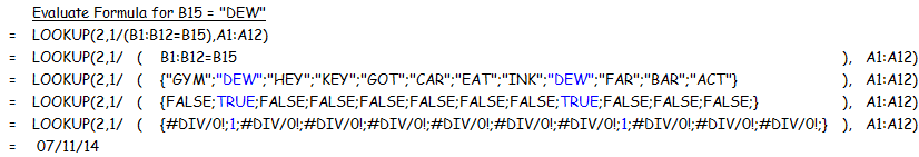
My 1st summary chart (moving from top to bottom) combines what is displayed in each of the evaluation steps when the Evaluate Formula tool is applied to the above formula:

My 2nd summary chart (now moving from left to right) displays what I think is happening by setting B15 equal to the range B1:B12 and placing the result as the denominator in the term: 1/(B1:B12=B15):

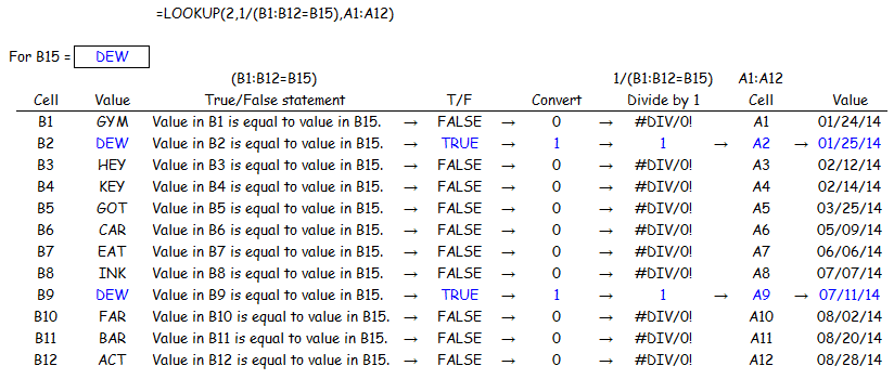I would appreciate any comments regarding the steps which are displayed.

byundt

The sequence of operations is great as far as you took it.

The remaining step requires understanding how LOOKUP works. LOOKUP compares the 2 in the first parameter to the values in the "Divide by 1" column. Not finding any match (or value larger than 2), it decides to focus attention on the very last match for a numeric data value. That means LOOKUP finds its match in row 9, and therefore returns the corresponding value from the "Value" column of your table: 07/11/14.

I purposely used the phrasing "corresponding value" instead of value from the same row. Although they are one and the same in this problem, had you been returning a value from a different worksheet, the "corresponding" value would obviously not be in the same row.

Brad

WeThotUWasAToad

ASKER

Extremely helpful. Thanks to everyone who contributed.