Mastering R Programming: Using Packages, Creating Objects, and Basic Matrix Functions


Published:
Browse All Articles > Mastering R Programming: Using Packages, Creating Objects, and Basic Matrix Functions
If you haven’t already, I encourage you to read the first article in my series to gain a basic foundation of R and R Studio. You will also find the links for downloading the programs there as well.
To begin, I want to mention a bit about the “packages” found in R. The incredible thing about R is that is a dynamically evolving language that gains functionality on a daily basis. Packages allow for anyone to compile functions and data sets together in one convenient bundle to extend to the base system functionality of R. There are two main repositories that host packages, CRAN and bioconductor. At the time of writing this article there are more than 9,000 individual packages available for use with R.
A majority of the packages will be installed from CRAN, so I will highlight the steps to install and load packages hosted there. The first thing you will need to do is to install the package, as an example we will install the ggplot2 (one of R’s most popular graphing packages). Once you have the package installed, you must then load it. The code is as follows:
Alternatively, utilizing R Studio, you can click the Packages tab in the bottom right window, click install, and enter ggplot2 in the Packages field (seen below):
![Screen-Shot-2015-07-21-at-12.05.38-PM.pn]()
![Screen-Shot-2015-07-21-at-12.11.37-PM.pn]() We will be using multiple different packages in this series but I will notify you which ones you need before I expect you to use them, just always remember to load the packages after you install it!
We will be using multiple different packages in this series but I will notify you which ones you need before I expect you to use them, just always remember to load the packages after you install it!
Concept 1: Objects
Now I would like to introduce you to a few of the functions and capabilities of R. Starting from where I left off in Article 1, we were observing that R can be used as a calculator:
Any time there is output in R, the result is assigned to a hidden named object .Last.value. Objects are one of the biggest foundations to R’s amazing functionality. Let’s try calling the object “Last value”
As you can see, the output is the output from our last line of executed code. This can come in handy later when you are performing multiple manipulations on different values. Now, lets create out own object.
The assignment operator (<-, you can also use “=”) dictates that the proceeding text gets assigned the information that follows the operator. I have also included the use of couple functions that return properties of the object.
Concept 2: Functions
Speaking of functions, lets take a look at some of the different built in functions of R. You could call simple math functions:
Notice all of these functions return the same value. There are multiple ways of manipulating data how best suits what you need with R. However, take note:
Now returns sqrt(2) because the last value outputted was 2, not 4 anymore. Keep that in mind if using a dynamic object like .Last.value. The cool thing is, you can even perform mathematics on objects!
Concept 3: Vectors
Vectors in R are single entities consisting of an ordered collection of items. To construct a vector you, the most common thing to do is to use the concatenate function c( ). To do so, seperate every new element in the vector by a comma. For example, you can have numeric vectors:
The first line of code only defines the vector, the second will allow you to see the output in R’s console window.
![Screen-Shot-2015-08-05-at-12.58.07-PM.pn]()
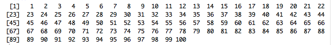
This output brings up an interesting point I want to make. The console window will output vectors, and other things like matrices and data sets, item by item. The []1] on the left shows the position of the current element you are looking at. So if for example, you have a vector of 100 elements, R will indicate to you which element starts the new row by a bracketed number (see the screenshot below for an example).
![Screen-Shot-2015-08-05-at-1.02.40-PM.png]()
You can make vectors full of items that are other functions:
Or even make vectors of strings:
Or have a vector with any combination of the former. Operations for determining properties of the vector include:
Other ways of creating vectors includes using the sequence and repetition functions [seq() & rep()]. You just have to remember to pass the arguments for by what interval the sequence forms or how many times to repeat the item.
Concept 4: Matrices
Perhaps one of my personal favorite things to do in R is matrix manipulation. Instead of having to put all my information into a matrix in my calculator I would rather use a program on the computer, like R, to carry out such calculations with ease. And the wonderful thing is that R has some incredible capabilities.
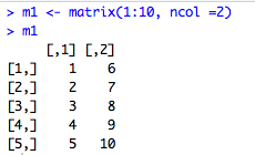
So lets make our first matrix:
Notice to populate the matrix I chose a sequence of number between 1 and 10, that is the 1:10 operation, and defined the number of columns I wanted, ncol=2. The output is displayed in a way that makes sense:
![Screen-Shot-2015-08-05-at-1.30.39-PM.png]()
Where the bracketed numbers on the left show the row position and the bracketed numbers on the top show the column position. Combined, this means that []3,2] is the element in row 3 column 2, which in our case is 8. We could also use the power of R to have it output this answer to us:
Or we can extract entire rows or columns:
Pretty trivial now, but could come in handy when you have large matrices and you need to perform operations on a specific element, row, or column.
It is important to mention there are some very handy arguments the matrix function can take, I will show you them in the following steps but for future reference you can call the help() function to see the types of arguments functions can take, for example if we need help with the matrix function:
I digress. Back to matrices. Here are some more examples of how to construct, index, and manipulate matrix elements:
Concept 5: Operators and Functions Using Matrices
Consider the square matrix:
We can perform some operations with this matrix such as the transpose, adding a constant to the matrix, multiplying by a constant, adding two matrices, multiplying by a vector or another matrix (listed respective order below):
All of these looking similar to normal mathematics, but say you want to use matrix multiplication, you need to use a special command:
If you notice, using an asterisk (*) and using the matrix multiplication (%*%) provide different answers. Be careful you use the correct one!
We can also create a diagonal matrix, take the inverse of a matrix, or find the determinant:
I encourage you to explore some of these different operations and functionalities yourself. There are so many things I haven’t touch upon that utilize these basic concepts but if you have any questions about what I have mentioned or how to go more in-depth, please leave a comment.
Also I would like to mention if there are any functionalities you would like to see in my upcoming articles, please let me know!
To begin, I want to mention a bit about the “packages” found in R. The incredible thing about R is that is a dynamically evolving language that gains functionality on a daily basis. Packages allow for anyone to compile functions and data sets together in one convenient bundle to extend to the base system functionality of R. There are two main repositories that host packages, CRAN and bioconductor. At the time of writing this article there are more than 9,000 individual packages available for use with R.
A majority of the packages will be installed from CRAN, so I will highlight the steps to install and load packages hosted there. The first thing you will need to do is to install the package, as an example we will install the ggplot2 (one of R’s most popular graphing packages). Once you have the package installed, you must then load it. The code is as follows:
install.packages("ggplot2")
library("ggplot2")Alternatively, utilizing R Studio, you can click the Packages tab in the bottom right window, click install, and enter ggplot2 in the Packages field (seen below):
Concept 1: Objects
Now I would like to introduce you to a few of the functions and capabilities of R. Starting from where I left off in Article 1, we were observing that R can be used as a calculator:
2+2Any time there is output in R, the result is assigned to a hidden named object .Last.value. Objects are one of the biggest foundations to R’s amazing functionality. Let’s try calling the object “Last value”
.Last.valueAs you can see, the output is the output from our last line of executed code. This can come in handy later when you are performing multiple manipulations on different values. Now, lets create out own object.
myobject <- 2+2
                      myobject
                      objects()
                      length(myobject)
is(myobject)The assignment operator (<-, you can also use “=”) dictates that the proceeding text gets assigned the information that follows the operator. I have also included the use of couple functions that return properties of the object.
Concept 2: Functions
Speaking of functions, lets take a look at some of the different built in functions of R. You could call simple math functions:
sqrt(4)
                      sqrt(2+2)
sqrt(myobject)Notice all of these functions return the same value. There are multiple ways of manipulating data how best suits what you need with R. However, take note:
sqrt(.Last.value)Now returns sqrt(2) because the last value outputted was 2, not 4 anymore. Keep that in mind if using a dynamic object like .Last.value. The cool thing is, you can even perform mathematics on objects!
(4*5)*myobjectConcept 3: Vectors
Vectors in R are single entities consisting of an ordered collection of items. To construct a vector you, the most common thing to do is to use the concatenate function c( ). To do so, seperate every new element in the vector by a comma. For example, you can have numeric vectors:
vector1 <- c(-10,-5,0,5,10)
vector1The first line of code only defines the vector, the second will allow you to see the output in R’s console window.
This output brings up an interesting point I want to make. The console window will output vectors, and other things like matrices and data sets, item by item. The []1] on the left shows the position of the current element you are looking at. So if for example, you have a vector of 100 elements, R will indicate to you which element starts the new row by a bracketed number (see the screenshot below for an example).
You can make vectors full of items that are other functions:
vector2 <- c(abs(-17),3/4,sqrt(-3),log(0),10^3)
vector2Or even make vectors of strings:
vector3 <- c(“Alpha”,”Beta”,”Gamma”)
vector3Or have a vector with any combination of the former. Operations for determining properties of the vector include:
mode(vector1)
                      range(vector1)
length(vector1)Other ways of creating vectors includes using the sequence and repetition functions [seq() & rep()]. You just have to remember to pass the arguments for by what interval the sequence forms or how many times to repeat the item.
seq(3,30,3)
                      rep(c(0:2,4,8), 3)
                      rep(c(0:2,4,8), each=3)
                      rep(c("Hi", "Ho"), 3)
                      rep(c("Hi", "Ho"), each=3)
                      rep(c(T,F), 3)
rep(c(T,F), each=3)Concept 4: Matrices
Perhaps one of my personal favorite things to do in R is matrix manipulation. Instead of having to put all my information into a matrix in my calculator I would rather use a program on the computer, like R, to carry out such calculations with ease. And the wonderful thing is that R has some incredible capabilities.
So lets make our first matrix:
m1 <- matrix(1:10, ncol =2)
m1Notice to populate the matrix I chose a sequence of number between 1 and 10, that is the 1:10 operation, and defined the number of columns I wanted, ncol=2. The output is displayed in a way that makes sense:
Where the bracketed numbers on the left show the row position and the bracketed numbers on the top show the column position. Combined, this means that []3,2] is the element in row 3 column 2, which in our case is 8. We could also use the power of R to have it output this answer to us:
m1[3,2]Or we can extract entire rows or columns:
m1[3,]
m1[c(4,5),]Pretty trivial now, but could come in handy when you have large matrices and you need to perform operations on a specific element, row, or column.
It is important to mention there are some very handy arguments the matrix function can take, I will show you them in the following steps but for future reference you can call the help() function to see the types of arguments functions can take, for example if we need help with the matrix function:
help(“matrix”)I digress. Back to matrices. Here are some more examples of how to construct, index, and manipulate matrix elements:
m2 <- matrix(1:10, nrow=2, byrow = TRUE)
                      m2
                      m3 <- matrix(1:12, ncol=4, byrow=TRUE)
                      m3
                      m3[3,]
                      m3 [,c(2,4)]
                      m3 [c(1,3),c(2,4)]
                      m3 [3,4] <- 0
m3Concept 5: Operators and Functions Using Matrices
Consider the square matrix:
m4 <- matrix(1:9,nrow=3)
m4We can perform some operations with this matrix such as the transpose, adding a constant to the matrix, multiplying by a constant, adding two matrices, multiplying by a vector or another matrix (listed respective order below):
t(m4)

                      m4 + 10

                      m4 * 4

                      m5 <- t(m4)
                      m4 + m5

                      v1 <- 1:3
                      v1

                      m4 * v1
m4 * m5All of these looking similar to normal mathematics, but say you want to use matrix multiplication, you need to use a special command:
m4 %*% m5If you notice, using an asterisk (*) and using the matrix multiplication (%*%) provide different answers. Be careful you use the correct one!
We can also create a diagonal matrix, take the inverse of a matrix, or find the determinant:
diag(c(3,2,1))
                      solve(matrix(c(8,9,6,7),nrow=2))
det(matrix(c(8,9,6,7),nrow=2))I encourage you to explore some of these different operations and functionalities yourself. There are so many things I haven’t touch upon that utilize these basic concepts but if you have any questions about what I have mentioned or how to go more in-depth, please leave a comment.
Also I would like to mention if there are any functionalities you would like to see in my upcoming articles, please let me know!
Have a question about something in this article? You can receive help directly from the article author. Sign up for a free trial to get started.
Comments (2)
Commented:
Commented:
I'm also a R enthusiastic and a self learner.
Just want to call your attention for the link to the next article. You didn't want to add it here in this article or it was on purpose?