Finding the Nth Lookup Value in an Excel List

By Patrick G. Matthews

Introduction

Excel users often need to perform a "lookup" operation against a table or list.  For example, one may have a table of geographical regions in one column, and in another column have the shipping rate applicable to each region.  The user can then create a formula that uses the region as an input, and returns the shipping rate that applies for that region.

Typically, the user must retrieve the value that applies to the first match in the lookup table.  In this case, Excel has two built-in functions that perform the job very well: VLOOKUP and INDEX.  However, in cases for which we may need the "Nth" value, where N may not equal 1, you need more complex expressions.  This article describes a general technique for retrieving the value corresponding to the Nth match, whether N is measured as "top to bottom", or as "bottom to top".

This article also demonstrates how to perform lookup operations when finding a match depends on two, three, or more criteria—a task which cannot be completed using the typical VLOOKUP or INDEX approach.

Sample File

The following sample file contains data used for each of the "Nth lookup" example in this article:

Nth-Match.xlsx

The file contains two worksheets:

Find First Match from the Top: VLOOKUP or INDEX/MATCH

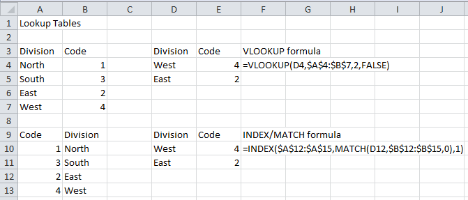
Most often, when you must return a value from a lookup table, you are looking for the first (or only!) match, based on a single criterion.  Consider the following lookup tables, in which we associate a Region with a Code:


In each case, we could construct a formula to retrieve the Code associated with any given Region.

In the first example, the index column, Region, is to the left of the column whose values we want to return (Code).  This being the case, many Excel users would build a VLOOKUP formula to retrieve the value, as noted in the image above.  (For anyone unfamiliar with the VLOOKUP function, please see this article on troubleshooting VLOOKUP expressions.

In the second lookup table, the index column, Region, is to the right of the Code column, and so VLOOKUP cannot be used.  In such a case, the next best alternative would be to use a combination of the INDEX and MATCH functions.

In the pictured example, the MATCH function looks for the indicated value, "West", in the range B12:B15, and if found it returns that value's ordinal position in the array.  For example, "West" was the fourth element in B12:B15, so in this case MATCH returned the value 4.

However, the following scenarios require a different approach:

Finding the Nth Match, Single Criterion

Now consider a more complex scenario, in which we may have to retrieve the second, third, fourth, or even "Nth" value from the lookup table, where "N" may even be a variable supplied by range reference.  In such cases, the simple VLOOKUP or INDEX/MATCH constructions will not do, so a different approach is required.

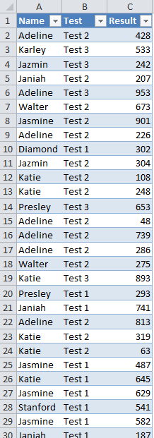
Consider the following scenario, in which we have test results for various participants.  There are three different forms for the test, and each participant may have taken the test several times:


Finding the first result in the table for a given participant or for a given test form would be easy, using either VLOOKUP or INDEX/MATCH, as seen above.  However, suppose you want to return the second or third result as well?  For this, a more complex approach is required.

For example, to find the third result from the top (irrespective of test form) for participant Adeline, use the following formula:

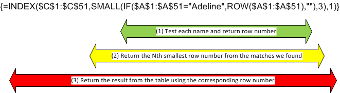
{=INDEX($C$1:$C$51,SMALL(IF($A$1:$A$51="Adeline",ROW($A$1:$A$51),""),3),1)}

This is an array formula, so do not type the curly braces ("{}"), and use Ctrl+Shift+Enter instead of Enter to complete the formula.  Excel will then display the curly braces to show that it is an array formula and not a scalar formula.

To see how this works, take it from the inside out:


The inner IF() expression, marked (1) above, evaluates each cell in A1:A51 to see if the value of the cell equals "Adeline".  If it does, then it returns the row number for that cell to the array; if not, then it returns a zero length string ("").  Thus, the array looks like this:

{"",2,"","","",6,"","",9,"","","","","",15,16,17,"",…}

That array gets passed to the SMALL() function, marked (2) above.  SMALL() takes in an array, and returns the kth smallest numeric value from that array (in this formula, k = 3).  It ignores non-numeric values.  Thus, the SMALL() expression returns 9, as it is the third smallest numeric value in the array.  If the value included for k in this expression exceeds the number of numeric values in the array, then the expression returns a #NUM! error.

Now, to get the answer, use INDEX(), marked (3) above, to return the indicated value from Column C.  If the SMALL() expression returned an error (because there were not enough numeric values in the array), that error will flow up to the INDEX() expression as the answer.

For example, to find the third result from the bottom (again irrespective of test form) for participant Adeline, use a similar array formula, exchanging the SMALL() function for the LARGE() function:

{=INDEX($C$1:$C$51,LARGE(IF($A$1:$A$51="Adeline",ROW($A$1:$A$51),""),3),1)}

Using the attached sample file, the LARGE() expression finds 22 as the third-largest numeric value in the array, and the corresponding result for Row 22 in the source data is 813.

Finding the Nth Match, Multiple Criteria

The array formula approach described above can be extended to cover matching on multiple criteria.  For example, to find the third result for participant "Adeline" and test form "Test 2", use the following array formula:

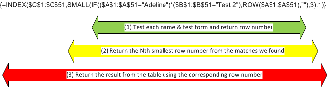
{=INDEX($C$1:$C$51,SMALL(IF(($A$1:$A$51="Adeline")*($B$1:$B$51=”Test 2"),ROW($A$1:$A$51),""),3),1)}

As above, this is an array formula, so do not type the curly braces ("{}"), and use Ctrl+Shift+Enter instead of Enter to complete the formula.  Excel will then display the curly braces to show that it is an array formula and not a scalar formula.

Evaluating this array formula from the inside out:


The inner IF() expression, marked (1) above, evaluates each pair of cells in A1:A51 and B1:B51 to see if the value of the cell from Column A equals "Adeline" and the value from Column B equals "Test 2".  If both tests are true, then it returns the row number for that cell to the array; if not, then it returns a zero length string ("").  Thus, the array looks like this:

{"",2,"","","","","","",9,"","","","","",15,16,17,"",…}

Note that we determine whether both tests are true my multiplying the results of the individual tests.  This exploits some special features of how Excel handles Boolean (true / false) values:

This approach is extensible to any number of criteria:

{=INDEX($C$1:$C$51,SMALL(IF((<criterion 1>)*(<criterion 2>)*(<criterion 3>)*…*(criterion Z>),ROW($A$1:$A$51),""),3),1)}

The behavior of the SMALL() expression marked as (2) and the INDEX() expression marked as (3) is identical to that described in the single criterion section above.  Also as with the single criterion approach, to select the Nth item from the bottom of the list, simply use the LARGE() function instead of the SMALL() function.

Error Handling

Note that when looking for the Nth match, from the top or the bottom, if your value for "N" exceeds the number of cells matching your criterion, the formulae above will return a #NUM! error.  This is because the SMALL() and LARGE() functions produce this error when the second argument exceeds the number of numeric values in the array being tested.

In Excel 2007 or later, to substitute an alternate value in this scenario, use the IFERROR function to trap the error:

{=IFERROR(INDEX($C$1:$C$51,SMALL(IF($A$1:$A$51="Adeline",ROW($A$1:$A$51),""),3),1),"<N/A>")}

In Excel 2003 or earlier, there is no IFERROR() function, so instead use:

{=IF(ISERROR(INDEX($C$1:$C$51,SMALL(IF($A$1:$A$51="Adeline",ROW($A$1:$A$51),""),3),1)),"<N/A",INDEX($C$1:$C$51,SMALL(IF($A$1:$A$51="Adeline",ROW($A$1:$A$51),""),3),1))}

Using Tables and Structured References for Nth Lookup

Tables are a new feature implemented in Excel 2007, and are extremely useful for storing data for analysis.  If your lookup data are stored in a Table, then you can use structured references instead of fixed ranges in any of the "Nth lookup" formulae shown above.

For example, to find the third result from the top (irrespective of test form) for participant Adeline, the following formula uses fixed range references:

{=INDEX($C$1:$C$51,SMALL(IF($A$1:$A$51="Adeline",ROW($A$1:$A$51),""),3),1)}

To use structured references from a Table instead, use:

{=INDEX(MyTable[[#All],[Result]],SMALL(IF(MyTable[[#All],[Name]]=$G4,ROW(MyTable[[#All],[Name]]),""),N$3),1)}

While the second formula is longer (albeit functionally identical to the original formula), and the syntax for structured references may be unfamiliar, the structured references offer two very significant advantages:

The worksheet "Using Table" in the attached sample file contains further examples on using structured references.


=-=-=-=-=-=-=-=-=-=-=-=-=-=-=-=-=-=-=-=-=-=-=-=-=-=-=-=-=-=-=-=-=-=-=-=-=-=-=-=-=
If you liked this article and want to see more from this author,  please click here.

If you found this article helpful, please click the Yes button near the:

      Was this article helpful?

label that is just below and to the right of this text.   Thanks!
=-=-=-=-=-=-=-=-=-=-=-=-=-=-=-=-=-=-=-=-=-=-=-=-=-=-=-=-=-=-=-=-=-=-=-=-=-=-=-=-=