

Browse All Articles > The 'Art' of Formatting - Excel Conditional Formatting
Every day, more and more users are turning to Excel for their data analysis needs.
Starting with Excel 2007 and fully taking shape in Excel 2010, Microsoft introduced a quick access link to create Conditional Formatting Rules. One major advantage in Excel is to be able to highlight and identify data at a glance, without the need to constantly Filter or Sort. Do you need the ability to change data frequently and want those values to automatically populate the appropriate formatting?
Starting with a new Excel Workbook, we will take some very basic data and make it stand out with Conditional Formatting.
In this example sheet, we start formatting information for at a glance reporting based on the criteria we define.
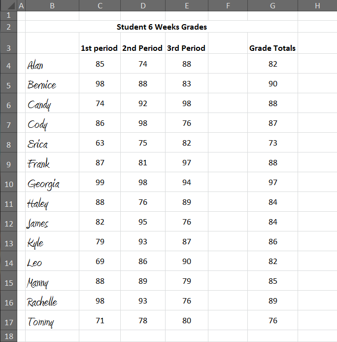
![Basic Sheet - Data with No Formatting]()
Here, we can see a Student listing with their respective Grades in each Class.
Based on this School's criteria, the following is how we will format the sheet:
1. Any Grade 90 and above is an "A"
2. Any Grade 80 to 89 is a "B"
3. Any Grade 70 to 79 is a "C"
4. Any Grade 69 or below is a Failing Grade.
Using this known information (our criteria) we will begin to format our Data.
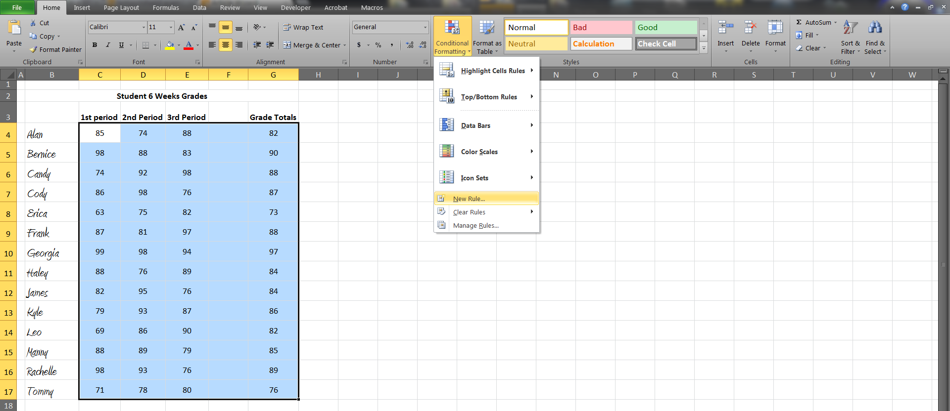
In this example, we will be selecting the range of cells from C4 to G17. With this data highlighted, we will access the Home Tab and select the Conditional Formatting Icon and then select the New Rule option, as shown below:
![New Conditional Formatting Rule]()
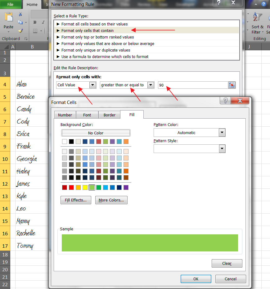
In this new window, we will make the following selections:
1. Format only cells that contain
2 Cell Value
3. greater than or equal to
4. 90 our value for an "A" Grade
5. Select the formatting that you would like to see by selecting the "Format..." button. Here I am using a green cell fill.
![Formatting Rule]()
Select OK for each window and you will start to see your formatting take affect.
Repeating the steps above, we will set up each formatting Rule. For Grades "B" and "C" and "D", we will replace Step 3 above with "less than or equal to".
NOTE: Even though logically this may seem confusing, Excel is able to differentiate which data falls under which value. For example, if we set the following formatting Rules where Rule 1 = less than or equal to 100; Rule 2 = less than or equal to 80; and Rule 3 = less than or equal to 50 - we can now enter the value "64" and Conditional Formatting will apply Rule 2, even though it can logically fall under Rule 1 as well.
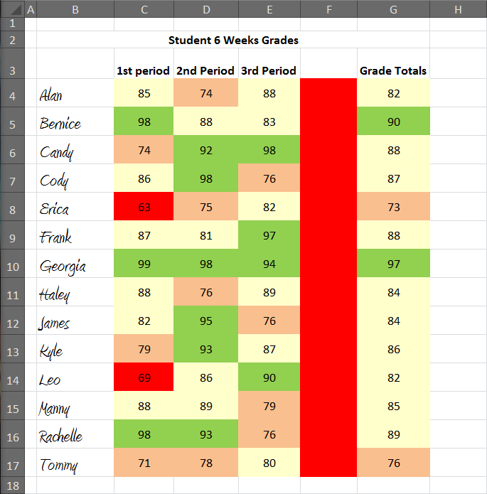
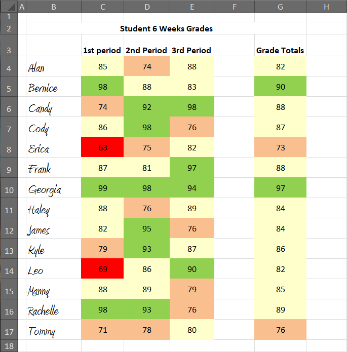
As you can see now, our data that we selected is no formatted based on the criteria we set up under Conditional Formatting:
![Conditionally Formatted Data]()
Removing Conditional Formatting
You will notice that since Column F was included when we selected our data range earlier, this field is also subjected to the Conditional Formatting. To remove this formatting for this Column only, we will select the entire Column by clicking the "F" header, selecting the Conditional Formatting Icon, hovering over the Clear Rules option and then selecting "Clear Rules from Selected Cells".
![Removed Formatting]()
Extra Formatting Options
When filling out your spreadsheets, keep in mind all of the options that Excel's Conditional Formatting has available to you, each option having more sub-options available:
Using Formulas
Excel also has the option to use formulas for Conditional Formatting. The most common formulas will be of the Formula Is option, where you enter formulas that result in either a TRUE or FALSE logical value returned.
Rules Manager
To Edit, Delete or create any Rules from the Rules Manager, we have two options:
1. Select the cells that you are wanting to Edit, Delete Formatting from or Create new Formatting for, choose the Conditional Formatting Icon and select Manage Rules. Here, you will be shown all Rules that pertain to your cell selection.
2. Without having to select any cells, access the Rules Manager as above; however, change the drop-down box option to show Rules for the entire worksheet as well as the Rules for each Sheet in the workbook.
For more information on Conditional Formatting, visit the Microsoft Office Support Pages.
I have also posted this Article on Experts Exchange blog : https://www.experts-exchange.com/blogs/ThinkSpaceSolutions/B_7007-The-'Art'-of-Formatting-Excel-Conditional-Formatting.html
Starting with Excel 2007 and fully taking shape in Excel 2010, Microsoft introduced a quick access link to create Conditional Formatting Rules. One major advantage in Excel is to be able to highlight and identify data at a glance, without the need to constantly Filter or Sort. Do you need the ability to change data frequently and want those values to automatically populate the appropriate formatting?
Starting with a new Excel Workbook, we will take some very basic data and make it stand out with Conditional Formatting.
In this example sheet, we start formatting information for at a glance reporting based on the criteria we define.
Here, we can see a Student listing with their respective Grades in each Class.
Based on this School's criteria, the following is how we will format the sheet:
1. Any Grade 90 and above is an "A"
2. Any Grade 80 to 89 is a "B"
3. Any Grade 70 to 79 is a "C"
4. Any Grade 69 or below is a Failing Grade.
Using this known information (our criteria) we will begin to format our Data.
In this example, we will be selecting the range of cells from C4 to G17. With this data highlighted, we will access the Home Tab and select the Conditional Formatting Icon and then select the New Rule option, as shown below:
In this new window, we will make the following selections:
1. Format only cells that contain
2 Cell Value
3. greater than or equal to
4. 90 our value for an "A" Grade
5. Select the formatting that you would like to see by selecting the "Format..." button. Here I am using a green cell fill.
Select OK for each window and you will start to see your formatting take affect.
Repeating the steps above, we will set up each formatting Rule. For Grades "B" and "C" and "D", we will replace Step 3 above with "less than or equal to".
NOTE: Even though logically this may seem confusing, Excel is able to differentiate which data falls under which value. For example, if we set the following formatting Rules where Rule 1 = less than or equal to 100; Rule 2 = less than or equal to 80; and Rule 3 = less than or equal to 50 - we can now enter the value "64" and Conditional Formatting will apply Rule 2, even though it can logically fall under Rule 1 as well.
As you can see now, our data that we selected is no formatted based on the criteria we set up under Conditional Formatting:
Removing Conditional Formatting
You will notice that since Column F was included when we selected our data range earlier, this field is also subjected to the Conditional Formatting. To remove this formatting for this Column only, we will select the entire Column by clicking the "F" header, selecting the Conditional Formatting Icon, hovering over the Clear Rules option and then selecting "Clear Rules from Selected Cells".
Extra Formatting Options
When filling out your spreadsheets, keep in mind all of the options that Excel's Conditional Formatting has available to you, each option having more sub-options available:
Format all cells based on their values:
Format only cells that contain:
Format only top or bottom ranked vales
Format only values that are above or below average
Format only unique or duplicate values
Using Formulas
Excel also has the option to use formulas for Conditional Formatting. The most common formulas will be of the Formula Is option, where you enter formulas that result in either a TRUE or FALSE logical value returned.
Rules Manager
To Edit, Delete or create any Rules from the Rules Manager, we have two options:
1. Select the cells that you are wanting to Edit, Delete Formatting from or Create new Formatting for, choose the Conditional Formatting Icon and select Manage Rules. Here, you will be shown all Rules that pertain to your cell selection.
2. Without having to select any cells, access the Rules Manager as above; however, change the drop-down box option to show Rules for the entire worksheet as well as the Rules for each Sheet in the workbook.
For more information on Conditional Formatting, visit the Microsoft Office Support Pages.
I have also posted this Article on Experts Exchange blog : https://www.experts-exchange.com/blogs/ThinkSpaceSolutions/B_7007-The-'Art'-of-Formatting-Excel-Conditional-Formatting.html
Have a question about something in this article? You can receive help directly from the article author. Sign up for a free trial to get started.
Comments (0)