

Browse All Articles > Creating an Efficient Dashboard in Excel
I produce a dashboard every day on a wealth of data, utilizing numerous graphs. Being that my graphs were based on a rolling 30 days’ worth of data, I was wasting a good amount of time updating all the data series in each of my graphs to start and end one row down (to include the new date’s data row and drop the last row).
Figuring there must be a way to have Excel do the nitty-gritty for me, I developed the following system, which allows me to simply add the new data each day and watch the graphs update themselves! Following is a simplified data set and 7-day dashboard to illustrate the basics:
![Article-1.png]()
![Article-2.png]()
![Article-3.png]()
Notes:
If you hide your helper columns, the graphs will appear blank. So, as visually useless as they are, it would be best to stash them in their own tab, or far to the right of something like the graphs, so they are unseen, but still referable.
If your dashboard is not daily, or is not produced regularly, you can always make the End Date a value you enter manually, which I do for certain weekly or monthly datasets.
If you decide to change the arrangement of your original dataset (the Widget Data tab in the example)—e.g. inserting or deleting columns—your helper columns will not follow suit. They will still be looking for data in, say, the sixth column. So be aware of any reformatting you do.
Figuring there must be a way to have Excel do the nitty-gritty for me, I developed the following system, which allows me to simply add the new data each day and watch the graphs update themselves! Following is a simplified data set and 7-day dashboard to illustrate the basics:
- Create a dynamic data set by using VLOOKUP
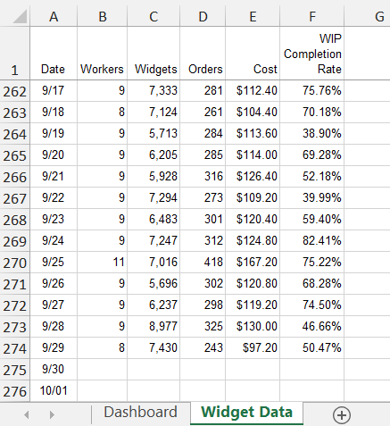
- My graphs need to show yesterday’s data and the 6 days prior, based on the data updated daily in my “Widget Data” tab:
I created four helper columns (in this case on the same tab as my graphs, though you can put them anywhere you find best suits your needs):
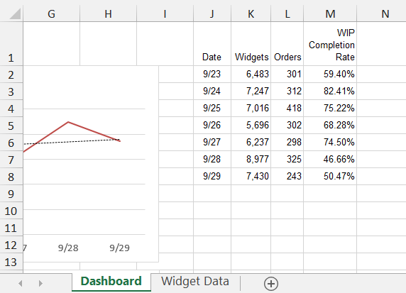
Because I want my dashboard graphs to update based on date, the first helper column (J) has the dates I want displayed (yesterday and the six days preceding that).
Cell J8 has the following formula: =(TODAY())-1
This returns yesterday’s date.
Cell J7: =J8-1
Cell J6: =J7-1
And so forth.
- The next three helper columns employ the VLOOKUP formula to identify the data on the Widget Data tab that corresponds to my daily-changing Column J.
Cell K2: =VLOOKUP($J2,'Widget Data'!$A$2:$D$2000,3,FALSE)
This formula is reading the date in J2, looking for its matching date in the leftmost column of the Range of A2:D200, and returning the data in the 3rd column within that range (in this case, C). “FALSE” signifies that I need Excel to find an exact match to the date I provide in J2 (“TRUE” would return the closest match within the leftmost column).
My use of the $ before J, A and D is so that I can drag the formula across columns to L and M and still have it looking for the same helper column data, within the same range. I will then only have to update the return column in the formula.
Cell L2: =VLOOKUP($J2,'Widget Data'!$A$2:$F$2000,4,FALSE)
Cell M2: =VLOOKUP($J2,'Widget Data'!$A$2:$F$2000,6,FALSE)
I manually changed the formula to look at columns 4 and 6, respectively, within the range.
My use of the $ in front of 2 and 2000 is so that I can then drag the formulas down to the next 6 rows and not shift the range down successively (this could be dangerous with bigger dashboards or smaller static data sets).
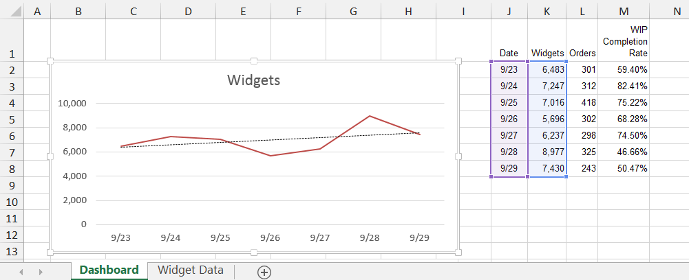
- Create graphs that look to your dynamic data set.
Notes:
If you hide your helper columns, the graphs will appear blank. So, as visually useless as they are, it would be best to stash them in their own tab, or far to the right of something like the graphs, so they are unseen, but still referable.
If your dashboard is not daily, or is not produced regularly, you can always make the End Date a value you enter manually, which I do for certain weekly or monthly datasets.
If you decide to change the arrangement of your original dataset (the Widget Data tab in the example)—e.g. inserting or deleting columns—your helper columns will not follow suit. They will still be looking for data in, say, the sixth column. So be aware of any reformatting you do.
Have a question about something in this article? You can receive help directly from the article author. Sign up for a free trial to get started.
Comments (2)
Commented:
Author
Commented:https://www.experts-exchange.com/Software/Office_Productivity/Office_Suites/MS_Office/Excel/A_2637-Six-Reasons-Why-Your-VLOOKUP-or-HLOOKUP-Formula-Does-Not-Work.html