Six Reasons Why Your VLOOKUP or HLOOKUP Formula Does Not Work


Published:
Browse All Articles > Six Reasons Why Your VLOOKUP or HLOOKUP Formula Does Not Work
by Patrick G. Matthews
VLOOKUP is a tremendously useful function that allows you to "fetch" data from a specified rectangular range (the "lookup table"); this range can be on the same worksheet, a different worksheet in the same workbook, or even in a different workbook entirely.
In a VLOOKUP call, Excel will search in the left-most column of the lookup table for a sought-for value (or if an exact match is not specified, then the closest value not exceeding that sought-for value), and then return the value in the Nth column from that row in the lookup table.
However, from time to time, you may find that your VLOOKUP formula is returning an error, or is returning an incorrect value. In my experience, there are six main causes for this:
This article will present a brief primer on VLOOKUP syntax, and then address each of these causes in turn.
Lastly, this article will also provide suggestions on how to handle errors returned by the VLOOKUP function.
Note: While VLOOKUP is the focus for this article, the same error conditions apply for the similar function HLOOKUP, which instead searches the first row of a lookup table, and then returns the value in the Nth row of the column where the match is found. Since VLOOKUP is used more frequently than HLOOKUP, the examples in this article will use VLOOKUP.
The VLOOKUP function takes four arguments:
When writing a VLOOKUP formula, please keep the following in mind:
The image below shows a few basic examples of VLOOKUP formulae:
![Basic Example]()
In that image:
Note: Elsewhere in this article, where I refer to a so-called "close match", I am referring to VLOOKUP's behavior when range_lookup is omitted or TRUE, and thus VLOOKUP is looking for the greatest value that is less than or equal to the value being sought.
As noted above, if the optional fourth argument, range_lookup, is omitted or is TRUE, then VLOOKUP will look for a "close" match in the first column of the lookup table. Specifically, VLOOKUP will look for the greatest value that is less than or equal to the value being sought, and then return the value in the Nth column of that corresponding row.
This will work, and allows the user to set up a lookup table to accommodate a single return value for a range of sought-for values. However, as noted in the Quick VLOOKUP Syntax Primer section above, the data in the first column of the lookup table must be sorted ascending in order for this to work.
Consider the examples below:
![Data Not Sorted]()
In the first block, the items in the lookup table are not sorted correctly: code 7, violet, is listed out of order, and thus the formulae in G6 and G10 return an incorrect result. In the second block, the formulae all return the correct results, because that lookup table lists the items in the correct order.
To avoid this error, if you are using VLOOKUP to find a "close" match, always make sure that your lookup table is sorted properly.
Note: In these examples, if we used FALSE for range_lookup, then the sort order of the lookup table would not have mattered, and all the formulae would have returned the correct results. That is, when you set VLOOKUP to look for an exact match, the lookup table does not have to be sorted: it can be in any order, and VLOOKUP will return the correct result assuming an exact match exists (or an #N/A error if there is no match).
If you set VLOOKUP to use a "close" match (by omitting range_lookup, or setting it to TRUE), VLOOKUP will look for the greatest value in the first column of the lookup table that is less than or equal to the value being sought. However, if the value being sought is less than every value in that first column of the lookup table, VLOOKUP will return a #N/A error. I term this failure "value sought is before first range", and the example below illustrates how it can occur.
![Before First Range]()
In this case, in the first block, VLOOKUP returns an error when it looks for zero in the lookup table: the smallest value in the lookup table's first column is 1, and zero is less than 1.
In the second block, the formulae all return the correct answer, this time because all of the values being sought have a value in the lookup table less than or equal to themselves.
To avoid this error, if you are using VLOOKUP to find a "close" match, always make sure that your lookup table is sorted properly, and that the smallest value in your lookup table is less than or equal to the smallest value you could conceivably pass to VLOOKUP for the first argument (lookup_value).
If you use FALSE for the optional fourth argument (range_lookup), VLOOKUP will look for an exact match in the lookup table. If it finds an exact match, then it will return a value from the Nth column of the corresponding row; if not, VLOOKUP will return an #N/A error. The example below illustrates the result when you seek an exact match for a value that is not in the lookup table.
![No Match]()
In this case, the value 26 does not exist in the lookup table, and so VLOOKUP returns an error in G7.
A possible fix for this situation would be to omit the fourth argument, and thus revert to a "close" match, as is done in the second group. After doing this, VLOOKUP will return "violet" in G18:
(Of course, while that construction avoids the #N/A value, it does not follow that that was in fact the "correct" result: the user may still have needed an exact match.)
To avoid this error, first be sure to determine whether or not you do in fact need an exact match--if you do not truly need an exact match, then omit range_lookup or use TRUE to allow a "close" match (and then be sure that the lookup table is sorted properly). If you really do need to have an exact match, avoid this error by making sure that your lookup table contains every conceivable value that VLOOKUP may look for.
VLOOKUP is sensitive to data types, and so the data type for the lookup_value must match the data type for the values in the first column of your lookup table. If these data types are not consistent, your VLOOKUP formula will fail, and VLOOKUP will return an #N/A error. Consider the examples below.
![Data Type Mismatch]()
In these examples, the first VLOOKUP formula in each group returns an #N/A error because of a data type mismatch:
To avoid this error, always make sure that you use consistent data types for your lookup_value and the first column of your lookup table. Be especially careful when copying and pasting values from another application, or importing/exporting values from another application, as such values may often appear to be true numeric or date values, but actually be stored as text by Excel. Values that appear to be numbers or dates can be coerced into numbers or dates, such as by using the VALUE or DATEVALUE functions, or by using Paste Special to multiply each cell in a range by 1.
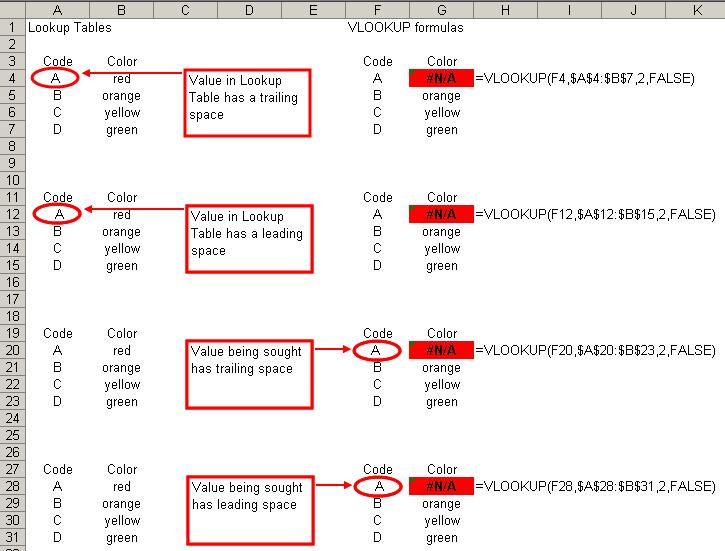
Extraneous spaces--leading spaces, trailing spaces, or additional spaces in between words--either in the lookup_value or in the values in the first column of the lookup table, can also cause VLOOKUP to return errors or unexpected values. Consider these examples below:
![Extraneous Spaces]()
In each case, an extraneous leading or trailing space, either in the lookup_value or in the lookup table, causes VLOOKUP to fail to find an exact match, and thus return an #N/A error. (In these cases, the "extraneous spaces" failure is thus a special case of the more general "no match" failure discussed previously.)
Extraneous spaces can also cause VLOOKUP to fail when using a "close" match, as extraneous spaces can:
To avoid this error, always make sure not to include leading or trailing spaces in your values, and to be consistent in hpw many spaces are used in between words in text entries. Extraneous spaces can be removed by using the TRIM function.
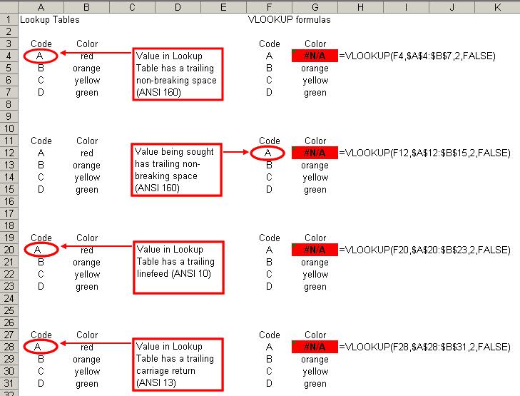
Occasionally, your lookup_value or the values in your lookup table may contain one or more "special" characters: characters in the ANSI character set that do not typically relate to a symbol (or forced white space) in printed output. The most commonly encountered "special characters" in this sense are the tab (ANSI 9), linefeed (ANSI 10), carriage return (ANSI 13), and non-breaking space (ANSI 160). The presence of any of these can cause your VLOOKUP formulae to fail, as in the examples below.
![Special Characters]()
In each case, the presence of one of these special characters caused an exact match to fail. In addition, as with extraneous spaces, special characters can also cause VLOOKUP to return an #N/A error or an unexpected result when looking for a close match.
To avoid this error, be careful not to include special characters in your lookup_value or in the lookup table. Be especially careful with text copied and pasted from a web page, as such content frequently uses non-breaking spaces. The CLEAN function will remove most special characters from a string, but will not remove the non-breaking space. Thus, you may have to use a formula such as this to remove special characters from a string:
=TRIM(CLEAN(SUBSTITUTE(A2,CHAR(160)," ")))
In this case, CLEAN removes most special characters, and SUBSTITUTE replaces any non-breaking spaces with regular spaces; the TRIM function finishes the job by removing any extraneous spaces that SUBSTITUTE may have introduced.
In some cases, avoiding an #N/A error in your VLOOKUP formula may not be feasible, but at the same time, you may still need to "handle" the error, either by preventing its display the error in your workbook, or by substituting another value for the error. The latter is especially important for cases in which other formulae may refer to the result of your VLOOKUP formula, as passing an error value to a dependent formula will cause that formula, and its dependents, to also produce errors.
In the first case, in which we want to "hide" an error value from view, perhaps the easiest way is through Conditional Formatting. In this case, we would use a formula-based rule to check the cell for an #N/A value. Thus, if the cell being checked is A2, then we would use the following formula:
=ISNA($A$2)
If, on the other hand, we needed to check every cell in the range A2:A100, then we would apply the following formula:
=ISNA(A2)
The relative range reference in that formula ensures that the Conditional Formatting rule applied to each cell refers to itself.
To "hide" the error, set the formatting such that the font color is the same as the cell's background color.
To instead substitute another value in the case of an error, we must adjust our basic VLOOKUP formula. Consider the following VLOOKUP formula:
=VLOOKUP(A2,Sheet2!A1:Z100,26,FALSE)
If Excel 2003 and earlier, if we want to make that formula return an alternate value in the event the lookup_value is not found in the lookup table, we could adjust that formula to use an IF expression to test for an error condition:
=IF(ISNA(VLOOKUP(A2,Sheet2!A1:Z100,26,FALSE)),"not found",VLOOKUP(A2,Sheet2!A1:Z100,26,FALSE))
In this formula, we first test for the error condition, and if it exists we return the alternate text "not found"; if there is no error, then we get the result of the VLOOKUP expression.
In Excel 2007 and later, this is somewhat simplified by using the new function IFERROR:
=IFERROR(VLOOKUP(A2,Sheet2!A1:Z100,26,FALSE),"not found")
In that construction, Excel returns the value in the first argument (in this case, a VLOOKUP expression) unless it is an error, in which case it returns the value in the second argument.
The sample file below contains all of the illustrated examples referred to in the various sections of this article.
VLOOKUP-Failure.xls
=-=-=-=-=-=-=-=-=-=-=-=-=-=-=-=-=-=-=-=-=-=-=-=-=-=-=-=-=-=-=-=-=-=-=-=-=-=-=-=-=
If you liked this article and want to see more from this author, please click here.
If you found this article helpful, please click the Yes button near the:
Was this article helpful?
label that is just below and to the right of this text. Thanks!
=-=-=-=-=-=-=-=-=-=-=-=-=-=-=-=-=-=-=-=-=-=-=-=-=-=-=-=-=-=-=-=-=-=-=-=-=-=-=-=-=
Introduction
VLOOKUP is a tremendously useful function that allows you to "fetch" data from a specified rectangular range (the "lookup table"); this range can be on the same worksheet, a different worksheet in the same workbook, or even in a different workbook entirely.
In a VLOOKUP call, Excel will search in the left-most column of the lookup table for a sought-for value (or if an exact match is not specified, then the closest value not exceeding that sought-for value), and then return the value in the Nth column from that row in the lookup table.
However, from time to time, you may find that your VLOOKUP formula is returning an error, or is returning an incorrect value. In my experience, there are six main causes for this:
Data are not sorted properly
The value sought comes before the first range
No matching data found in the lookup table
Data type mismatch
Extraneous spaces
Special characters
This article will present a brief primer on VLOOKUP syntax, and then address each of these causes in turn.
Lastly, this article will also provide suggestions on how to handle errors returned by the VLOOKUP function.
Note: While VLOOKUP is the focus for this article, the same error conditions apply for the similar function HLOOKUP, which instead searches the first row of a lookup table, and then returns the value in the Nth row of the column where the match is found. Since VLOOKUP is used more frequently than HLOOKUP, the examples in this article will use VLOOKUP.
Quick VLOOKUP Syntax Primer
The VLOOKUP function takes four arguments:
lookup_value is the value sought for in the first column of the lookup table
table_array is an array specifying the lookup table. table_array is usually a range, and that range need not be on the same worksheet--or even in the same workbook--as the cell where you enter the formula. table_array can also be a Name, or even an array constant
col_index_number specifies which column from the corresponding row is used for the return value. For example, if col_index_number = 3, then the value returned is the value in the third column of the lookup table
range_lookup is an optional argument. If this is FALSE, VLOOKUP looks for an exact match in the first column of the lookup table. If this is TRUE or omitted, VLOOKUP looks for the greatest value that is less than or equal to the value being sought
When writing a VLOOKUP formula, please keep the following in mind:
VLOOKUP is not case sensitive. Thus, for text matches, it does not matter whether you use lower-, upper-, or mixed case
VLOOKUP will not do data type conversions, so if the value being sought is numeric, then the first column of the lookup table should be numeric as well, and if the value being sought is text, then the first column of the lookup table should be text as well
If you omit, or use TRUE for range_lookup (i.e., you are looking for a "close match"), then you must be sure that the first column of the lookup table is sorted, ascending, or VLOOKUP may not return the correct result. However, if you use FALSE, there is no need to sort the lookup table
If you use FALSE for range_lookup, and the sought-for value is not in the first column of the lookup table, VLOOKUP will return a #N/A error
If you use FALSE for range_lookup, and if the values in the first column of the lookup table are text, you can use wild cards in lookup_value. To match zero or more characters use the asterisk, and to match a single character use the question mark. Thus, "R*" would match "red" or "rojo" or even simply "r", and "r??" would match "red" but neither "rojo" nor "r". To match the actual asterisk or question mark characters, precede them with a tilde. Thus, to match the actual sequence "r??", you would use "r~?~?"
If col_index_number is less than 1, or if it exceeds the number of columns in the lookup table, VLOOKUP will return an error (#VALUE! or #REF!, respectively)
The image below shows a few basic examples of VLOOKUP formulae:
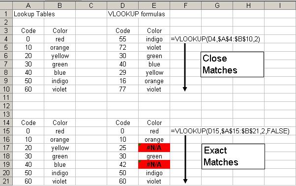
In that image:
In E4, E5, E8, E9, and E10, the formula returns "close" matches
In E6 and E7, while the formula is looking for a "close" match, the values sought for happen to have exact matches in the lookup table
In E15, E16, E18, E20, and E21, the formula found exact matches
In E17 and E19, the formula looked for, but did not find, exact matches
Note: Elsewhere in this article, where I refer to a so-called "close match", I am referring to VLOOKUP's behavior when range_lookup is omitted or TRUE, and thus VLOOKUP is looking for the greatest value that is less than or equal to the value being sought.
Data Not Sorted
As noted above, if the optional fourth argument, range_lookup, is omitted or is TRUE, then VLOOKUP will look for a "close" match in the first column of the lookup table. Specifically, VLOOKUP will look for the greatest value that is less than or equal to the value being sought, and then return the value in the Nth column of that corresponding row.
This will work, and allows the user to set up a lookup table to accommodate a single return value for a range of sought-for values. However, as noted in the Quick VLOOKUP Syntax Primer section above, the data in the first column of the lookup table must be sorted ascending in order for this to work.
Consider the examples below:
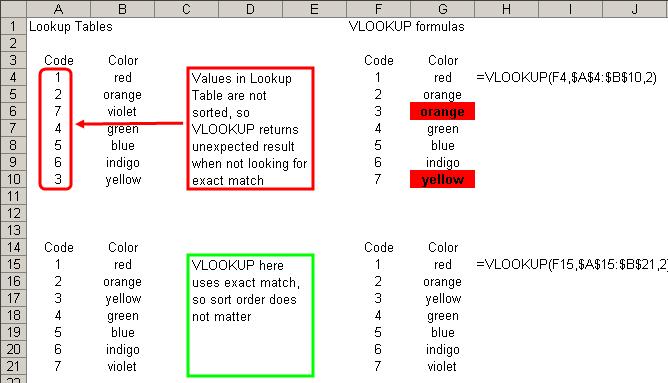
In the first block, the items in the lookup table are not sorted correctly: code 7, violet, is listed out of order, and thus the formulae in G6 and G10 return an incorrect result. In the second block, the formulae all return the correct results, because that lookup table lists the items in the correct order.
To avoid this error, if you are using VLOOKUP to find a "close" match, always make sure that your lookup table is sorted properly.
Note: In these examples, if we used FALSE for range_lookup, then the sort order of the lookup table would not have mattered, and all the formulae would have returned the correct results. That is, when you set VLOOKUP to look for an exact match, the lookup table does not have to be sorted: it can be in any order, and VLOOKUP will return the correct result assuming an exact match exists (or an #N/A error if there is no match).
Value Sought Is before First Range
If you set VLOOKUP to use a "close" match (by omitting range_lookup, or setting it to TRUE), VLOOKUP will look for the greatest value in the first column of the lookup table that is less than or equal to the value being sought. However, if the value being sought is less than every value in that first column of the lookup table, VLOOKUP will return a #N/A error. I term this failure "value sought is before first range", and the example below illustrates how it can occur.
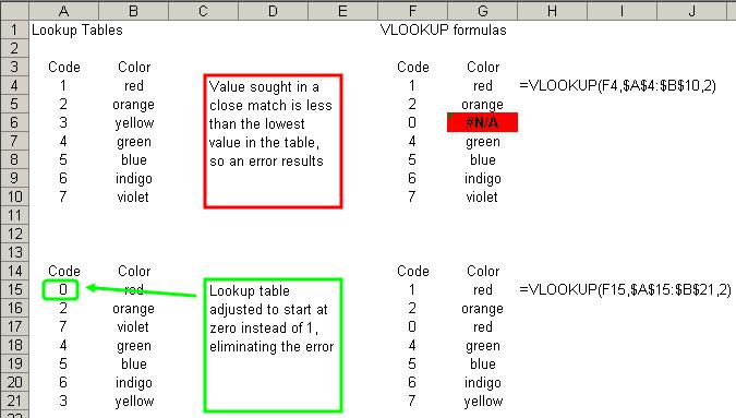
In this case, in the first block, VLOOKUP returns an error when it looks for zero in the lookup table: the smallest value in the lookup table's first column is 1, and zero is less than 1.
In the second block, the formulae all return the correct answer, this time because all of the values being sought have a value in the lookup table less than or equal to themselves.
To avoid this error, if you are using VLOOKUP to find a "close" match, always make sure that your lookup table is sorted properly, and that the smallest value in your lookup table is less than or equal to the smallest value you could conceivably pass to VLOOKUP for the first argument (lookup_value).
No Match in Lookup Table
If you use FALSE for the optional fourth argument (range_lookup), VLOOKUP will look for an exact match in the lookup table. If it finds an exact match, then it will return a value from the Nth column of the corresponding row; if not, VLOOKUP will return an #N/A error. The example below illustrates the result when you seek an exact match for a value that is not in the lookup table.
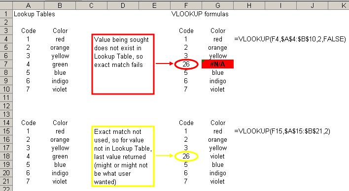
In this case, the value 26 does not exist in the lookup table, and so VLOOKUP returns an error in G7.
A possible fix for this situation would be to omit the fourth argument, and thus revert to a "close" match, as is done in the second group. After doing this, VLOOKUP will return "violet" in G18:
The sought-for value is 26
The greatest value in the lookup table that is less than or equal to 26 is the last, 7
The second column from that row of the lookup table contains "violet"
(Of course, while that construction avoids the #N/A value, it does not follow that that was in fact the "correct" result: the user may still have needed an exact match.)
To avoid this error, first be sure to determine whether or not you do in fact need an exact match--if you do not truly need an exact match, then omit range_lookup or use TRUE to allow a "close" match (and then be sure that the lookup table is sorted properly). If you really do need to have an exact match, avoid this error by making sure that your lookup table contains every conceivable value that VLOOKUP may look for.
Data Type Mismatch
VLOOKUP is sensitive to data types, and so the data type for the lookup_value must match the data type for the values in the first column of your lookup table. If these data types are not consistent, your VLOOKUP formula will fail, and VLOOKUP will return an #N/A error. Consider the examples below.
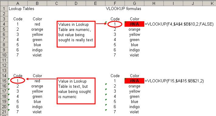
In these examples, the first VLOOKUP formula in each group returns an #N/A error because of a data type mismatch:
In G4, VLOOKUP returns an error because the lookup_value is "1" and not the number 1; since the values in the lookup table are numeric, there is a data type mismatch
In G15, VLOOKUP returns an error because the lookup_value is the number 1 and not "1"; since the values in the lookup table are text, there is a data type mismatch
To avoid this error, always make sure that you use consistent data types for your lookup_value and the first column of your lookup table. Be especially careful when copying and pasting values from another application, or importing/exporting values from another application, as such values may often appear to be true numeric or date values, but actually be stored as text by Excel. Values that appear to be numbers or dates can be coerced into numbers or dates, such as by using the VALUE or DATEVALUE functions, or by using Paste Special to multiply each cell in a range by 1.
Extraneous Spaces
Extraneous spaces--leading spaces, trailing spaces, or additional spaces in between words--either in the lookup_value or in the values in the first column of the lookup table, can also cause VLOOKUP to return errors or unexpected values. Consider these examples below:
In each case, an extraneous leading or trailing space, either in the lookup_value or in the lookup table, causes VLOOKUP to fail to find an exact match, and thus return an #N/A error. (In these cases, the "extraneous spaces" failure is thus a special case of the more general "no match" failure discussed previously.)
Extraneous spaces can also cause VLOOKUP to fail when using a "close" match, as extraneous spaces can:
Force what was intended to be a numeric value into a text value (and thus trip the "data type mismatch" failure);
Cause the lookup table to not be sorted correctly;
Lead VLOOKUP to incorrectly compare text strings (and thus return an expected value, or trigger the "before first range" failure
Et cetera.
To avoid this error, always make sure not to include leading or trailing spaces in your values, and to be consistent in hpw many spaces are used in between words in text entries. Extraneous spaces can be removed by using the TRIM function.
Special Characters
Occasionally, your lookup_value or the values in your lookup table may contain one or more "special" characters: characters in the ANSI character set that do not typically relate to a symbol (or forced white space) in printed output. The most commonly encountered "special characters" in this sense are the tab (ANSI 9), linefeed (ANSI 10), carriage return (ANSI 13), and non-breaking space (ANSI 160). The presence of any of these can cause your VLOOKUP formulae to fail, as in the examples below.
In each case, the presence of one of these special characters caused an exact match to fail. In addition, as with extraneous spaces, special characters can also cause VLOOKUP to return an #N/A error or an unexpected result when looking for a close match.
To avoid this error, be careful not to include special characters in your lookup_value or in the lookup table. Be especially careful with text copied and pasted from a web page, as such content frequently uses non-breaking spaces. The CLEAN function will remove most special characters from a string, but will not remove the non-breaking space. Thus, you may have to use a formula such as this to remove special characters from a string:
=TRIM(CLEAN(SUBSTITUTE(A2,
In this case, CLEAN removes most special characters, and SUBSTITUTE replaces any non-breaking spaces with regular spaces; the TRIM function finishes the job by removing any extraneous spaces that SUBSTITUTE may have introduced.
Error Handling for VLOOKUP
In some cases, avoiding an #N/A error in your VLOOKUP formula may not be feasible, but at the same time, you may still need to "handle" the error, either by preventing its display the error in your workbook, or by substituting another value for the error. The latter is especially important for cases in which other formulae may refer to the result of your VLOOKUP formula, as passing an error value to a dependent formula will cause that formula, and its dependents, to also produce errors.
In the first case, in which we want to "hide" an error value from view, perhaps the easiest way is through Conditional Formatting. In this case, we would use a formula-based rule to check the cell for an #N/A value. Thus, if the cell being checked is A2, then we would use the following formula:
=ISNA($A$2)
If, on the other hand, we needed to check every cell in the range A2:A100, then we would apply the following formula:
=ISNA(A2)
The relative range reference in that formula ensures that the Conditional Formatting rule applied to each cell refers to itself.
To "hide" the error, set the formatting such that the font color is the same as the cell's background color.
To instead substitute another value in the case of an error, we must adjust our basic VLOOKUP formula. Consider the following VLOOKUP formula:
=VLOOKUP(A2,Sheet2!A1:Z100
If Excel 2003 and earlier, if we want to make that formula return an alternate value in the event the lookup_value is not found in the lookup table, we could adjust that formula to use an IF expression to test for an error condition:
=IF(ISNA(VLOOKUP(A2,Sheet2
In this formula, we first test for the error condition, and if it exists we return the alternate text "not found"; if there is no error, then we get the result of the VLOOKUP expression.
In Excel 2007 and later, this is somewhat simplified by using the new function IFERROR:
=IFERROR(VLOOKUP(A2,Sheet2
In that construction, Excel returns the value in the first argument (in this case, a VLOOKUP expression) unless it is an error, in which case it returns the value in the second argument.
Sample File
The sample file below contains all of the illustrated examples referred to in the various sections of this article.
VLOOKUP-Failure.xls
=-=-=-=-=-=-=-=-=-=-=-=-=-
If you liked this article and want to see more from this author, please click here.
If you found this article helpful, please click the Yes button near the:
Was this article helpful?
label that is just below and to the right of this text. Thanks!
=-=-=-=-=-=-=-=-=-=-=-=-=-
Have a question about something in this article? You can receive help directly from the article author. Sign up for a free trial to get started.
Comments (21)
Commented:
My most annoying bug is that the vlookup will not refresh when copying the formula.
The lookup cell has changed, yet a number of records in the middle of my sheet do not update to the correct value!
Refresh does nothing...
Most annoying.
Commented:
Regards, Andreas
Commented:
Commented:
Commented:
Calin
View More