Forecasting in Excel 2016 for Windows and Mac

Excel 2016 has a handful of new functions to help you forecast numbers – typically sales data – more accurately than before. The older FORECAST function still exists for compatibility with worksheets created in older versions, but if you’re creating a new sheet, you’ll want to use one of these…

FORECAST.LINEAR: creates a straight-line forecast

FORECAST.ETS: estimates a trend using seasonality

FORECAST.ETS.SEASONALITY: shows the length of a seasonal cycle

FORECAST.ETS.CONFINT: the confidence interval of the estimate

FORECAST.ETS.STAT: calculates 8 statistical algorithms

These work the same in both the Windows and Mac versions of Excel 2016. Once you have the results, you can create a chart in the Windows version that shows the forecasts and expected margins of error. The Forecast Sheet chart isn’t available on the Mac edition of 2016, but you can still create a regular chart.

If you'd like to follow along, download this zip file and extract the workbook from it:

http://www.flisser.com/download/forecast-functions.zip

Straight Line Forecasting

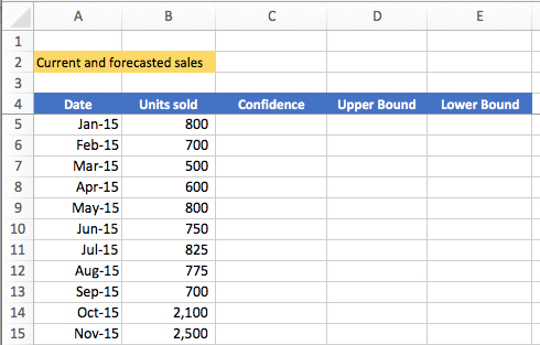
The workbook has two tabs: straight line and seasonality. Start with the straight line tab. This type of data doesn’t have a cycle, which means the sales don’t depend on the time of year.

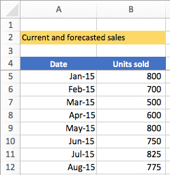
The sheet has two columns of monthly data: dates and units sold. You need dates and their corresponding numbers for all the forecasting functions.

The last date for which we have data is May 2017. We want to know what the units sold will be for June through December.

The syntax of a straight line forecast is:

=FORECAST.LINEAR(date to forecast to, range of current sales, range of current dates)

On this sheet, the range of current sales is A5:A33 and the current dates are in B5:B33. To make the calculations easier, I gave these range names of dates_sheet_1 and units_sheet_1. You can see all the range names for this workbook by clicking the Name Box in the upper left corner of the sheet. (If you want, click one of the names to select its range.)

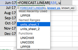
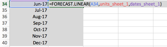
Click in B34 and calculate the first forecasted units, which is for June 2017. Enter the formula:

=FORECAST.LINEAR(A34, units_sheet_1, dates_sheet_1)

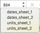
Hint: you don’t have to type the range names manually. When you start typing a name, Excel displays a list of hints. Select one:

Or press the F3 key on the keyboard (Fn + F3 on the Mac) to display the Paste Name box: a list of all range names on the sheet.

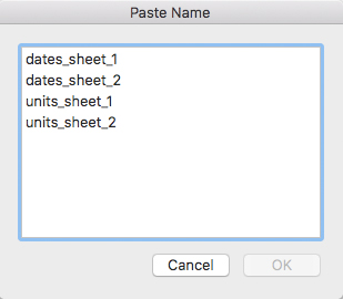
Double-click the one you want. (Do it twice when writing this formula: once to insert the units name and once to insert the dates name.)

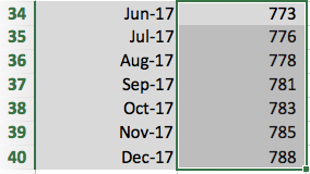
The function’s result should be 773. Use AutoFill to copy the formula down to the bottom:

Seasonal Forecasting

How do you forecast data if they are effected by the date? Typical examples are consumer electronics, where sales spike in the 4^th quarter of the year, and vacation rentals, where sales spike in the summer.

Notice the Seasonality sheet has 3 full years of data, and in each year, the units sold are significantly higher in the 4^th quarters. The seasonality function usually needs 3 years of data for good results.

The syntax for the Seasonality forecasting function has the same 3 arguments as the straight-line function, and 3 optional arguments:

=FORECAST.ETS(date to forecast to, range of current sales, range of current dates, [number of seasonal data points], [data completion], [aggregation])

ETS stands for Exponential Triple Smooth. Excel estimates the numbers based on trends and seasonality, giving the most weight to recent data, declining exponentially.

Optional arguments

Number of seasonal date points

If number of date points = 0, Excel assumes no seasonality

If number of date points = blank, Excel guesses the number of seasonal date points

Data completion

If you don't have a sales value for a period, choose 0 or 1

1: default. Excel will fill in the blank by averaging the previous and next values

0: missing values treated as zeros

Aggregation

If you have multiple values for the same period, what should Excel do? Options:

1=Average (default)

2=Count

3=Counta

4=Max

5=Median

6=Min

7=Sum

As in the previous sheet, I created range names for you to make this easier.

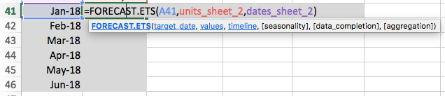
In B41, enter the formula, using the above techniques for inserting the range names. To keep it simple, you can leave out the optional arguments.

=FORECAST.ETS(A41, units_sheet_2, dates_sheet_2)

The result should be 926. Use AutoFill to copy the formula down to the bottom:

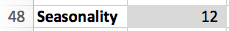
What’s the Seasonal Cycle?

To calculate how many months Excel sees in a cycle, use FORECAST.ETS.SEASONALITY.

The syntax is similar to FORECAST.ETS but with fewer arguments:

=FORECAST.ETS.SEASONALITY(range of current sales, range of current dates, [data completion], [aggregation])

In B48, enter the formula:

=FORECAST.ETS.SEASONALITY(units_sheet_2, dates_sheet_2)

The result is 12, meaning the formula sees 12 months in a cycle.

Confidence

How confident are we in the results? A Confidence Interval will tell us how much margin of error above and below the forecast we can expect.

The Confidence Interval function has similar syntax with 3 required arguments and 4 optional ones. The only new one you haven’t seen yet is the confidence level percent.

The syntax is:

=FORECAST.ETS.CONFINT(date to forecast to, range of current sales, range of current dates, [confidence level], [number of seasonal data points], [data completion], [aggregation])

The default confidence level is 95% (roughly 4 standard deviations).

Enter the formula in C41, accepting the default confidence level:

=FORECAST.ETS.CONFINT(A41,units_sheet_2,dates_sheet_2)

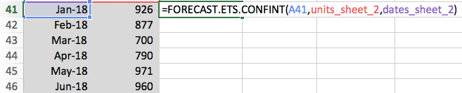
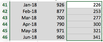
The result should be roughly 226. On the Home tab of the ribbon, use the Decrease Decimal button to remove the decimals.

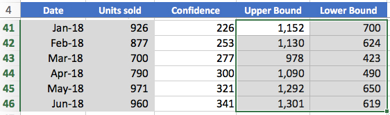
Let’s now add and subtract these numbers from the forecast to get a table of upper and lower results to expect.

In D41, enter this formula to add the confidence to the forecast and get the upper bound:

=B41+C41

In E41, enter this formula to subtract the confidence from the forecast and get the lower bound:

=B41-C41

Use AutoFill to copy both formulas down to the bottom:

Statistics

To see statistical relationships between the unit and date range, use FORECAST.ETS.STAT. It can return one of these 8 statistics, using the following code numbers in the function:

Alpha parameter of the ETS algorithm
Beta parameter of the ETS algorithm
Gamma parameter of the ETS algorithm
MASE metric
SMAPE metric
MAE metric
RMSE metric
Step size

The syntax is similar to the previous functions:

=FORECAST.ETS.STAT(range of current sales, range of current dates, statistic type, [seasonality], [data completion], [aggregation])

In B51, use code 2 to find the beta:

=FORECAST.ETS.STAT(units_sheet_2, dates_sheet_2, 2)

The result should be 0.1%.

Charting Forecasts

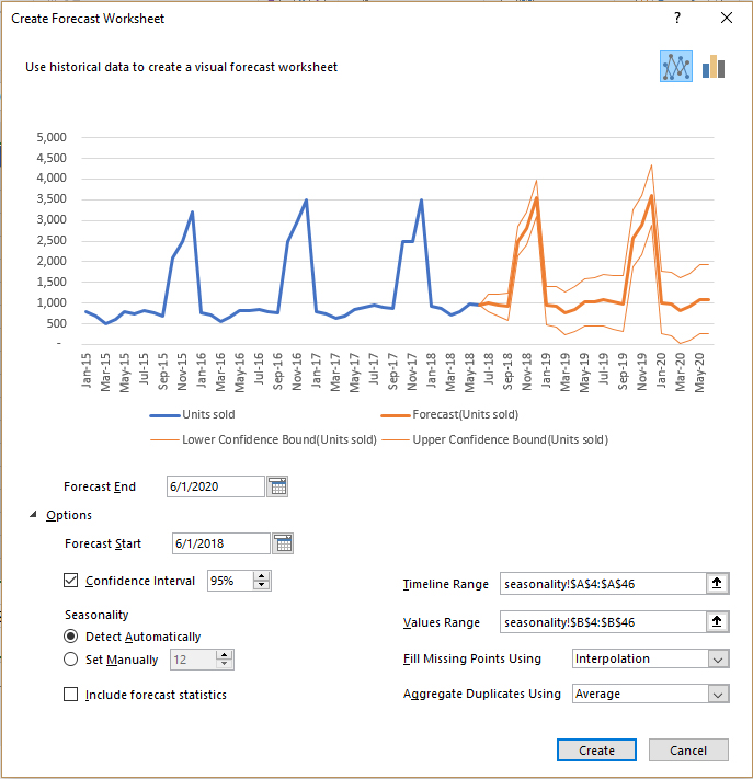
The Windows version of Excel 2016 has a button that places an interactive forecast chart on your sheet. On the ribbon, click the Data tab, then click the Forecast Sheet button.

On the bottom of the dialog, click Options to expand the dialog. Here, you have all the options the functions give you. Make your choices, then click the Create button to insert the chart.

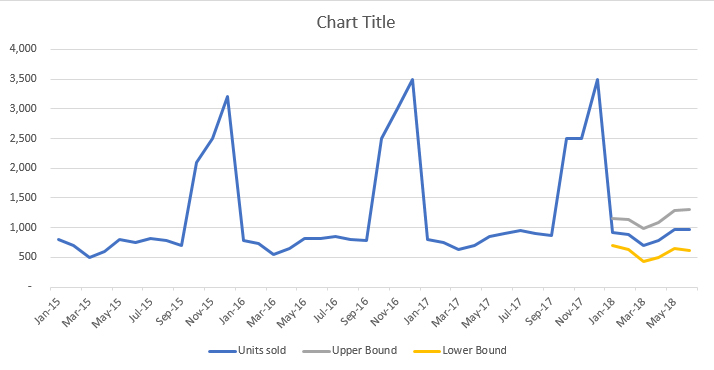
Although the Mac version of Excel 2016 doesn’t have this feature, you can still go to the Insert tab on the ribbon and insert a line chart: