Handling Duplicate Rows In Excel

I have seen that some experts have written articles on how to handle duplicate rows in Excel, such as:

• Eliminating duplicate data with Duplicate Master V2
• Excel VBA - How to delete duplicate inside the same cell

Those articles are quite impressive. However, I would just like to cover some of the scenarios and provide other relevant useful methods.

This article will cover the areas in:

1. Using Formula
2. Using Conditional Formatting
3. Keep only One Row (De-duping)
4. Keep only Duplicate Rows
5. Delete the Duplicate Rows
6. Move the Duplicate or Unique Rows to Another Sheet

To begin with this tutorial, you may probably want to download the source file here.

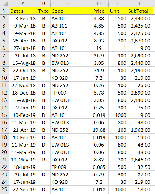
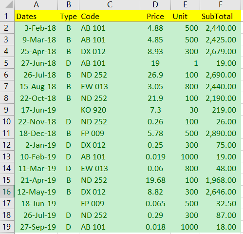
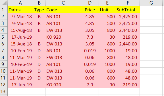
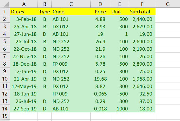
The source file consists of 6 columns and 24 rows of data.

---

Let's start the tutorial!

1. Using Formula

First, to identify the no of counts within a range, rows or columns, we could use the COUNTIF function. In case there is more than one condition to determine the selection, we would use the COUNTIFS function instead.

In this case, we would use the COUNTIFS function instead.

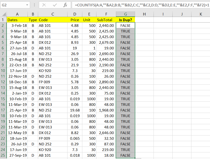
We can place the formula at cell G2. Since we are going to examine the duplicate data across all the columns, the formula that would be applied is:

=COUNTIFS(A:A,A2,B:B,B2,C:C,C2,D:D,D2,E:E,E2,F:F,F2)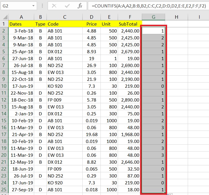

We can drag the formula down and you should see the result as below:


As you could see from the result:

• Values equals to 1 means the rows are unique.
• Values greater than 1 means the rows are not unique.

Do note that there are rows with value equals to  0. According to COUNTIFS documentation:

If the criteria argument is a reference to an empty cell, the COUNTIFS function treats the empty cell as a 0 value.

To resolve this issue, we would change the formula to:

=COUNTIFS(A:A,""&A2,B:B,""&B2,C:C,""&C2,D:D,""&D2,E:E,""&E2,F:F,""&F2)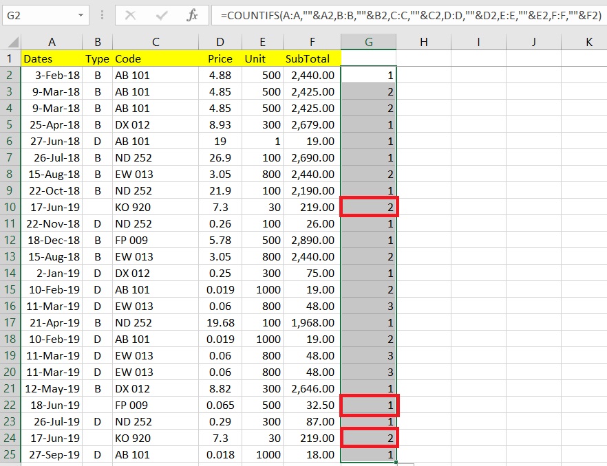

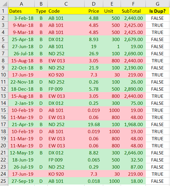
We will see the zero issue is now being resolved.


We could further enhance the formula so that it would return a True / False instead, like:

=COUNTIFS(A:A,""&A2,B:B,""&B2,C:C,""&C2,D:D,""&D2,E:E,""&E2,F:F,""&F2)>1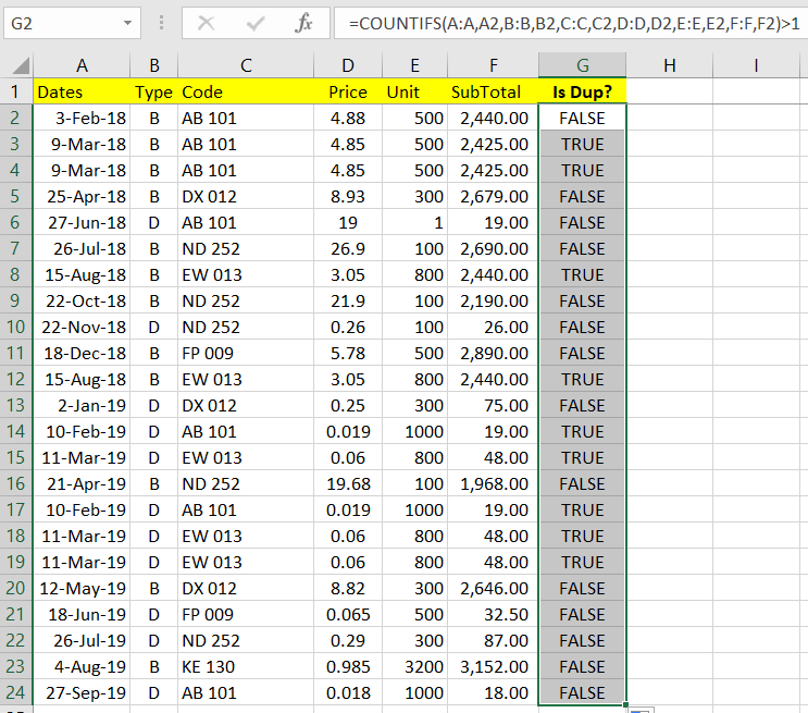

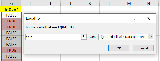
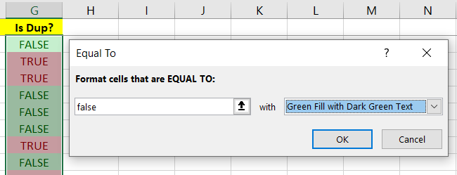
We can do the same by dragging the formula down.


To make it easier to identify the result, we can use Conditional Formatting to color the results.

Let's say:

• Green color for FALSE
• Red color for TRUE

So, the end result would be something as below:


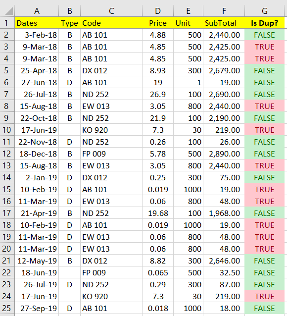
We will be re-using Conditional Formatting to highlight the duplicate rows in the next example.

2. Using Conditional Formatting

Conditional Formatting already got the existing wizard to highlight the duplicate values. But it only selected based on the value of individual cells.

Hence, this is not really is the effect we wanted in which it "selected" the whole row instead.


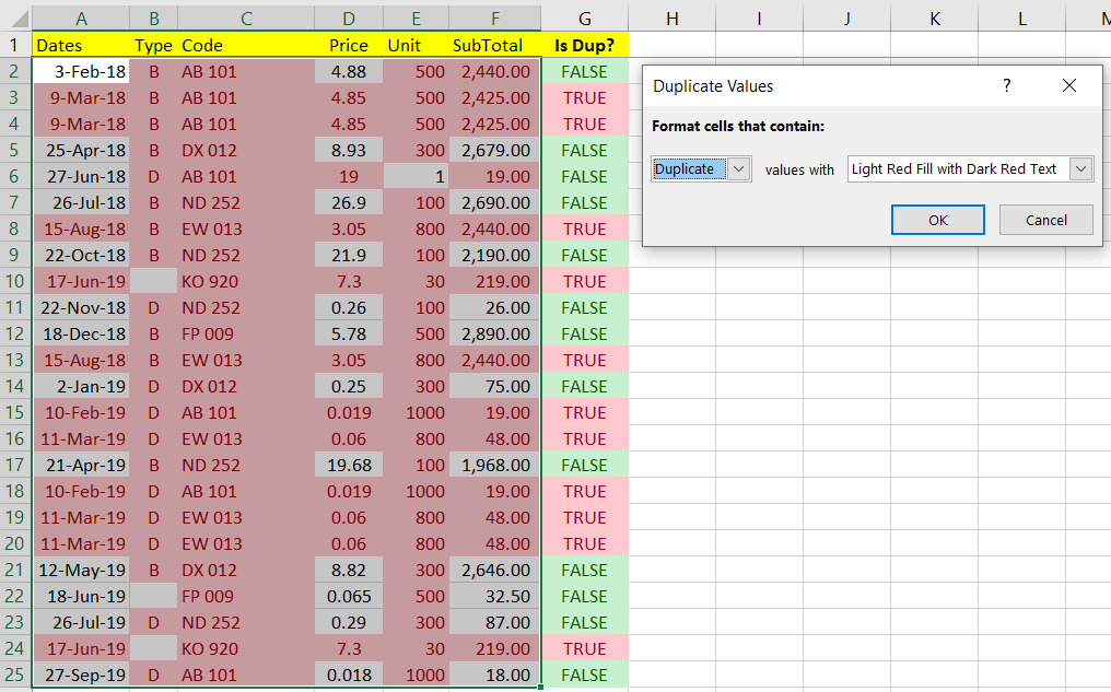
To better handle this scenario, we need to use Formula within Conditional Formatting instead.

I ) With Conditional Formatting - Method 1

To start, we can first create a pair of "dummy" conditional formatting at cell A2, which is to keep the color settings of Red and Green.

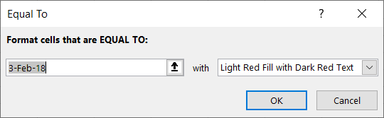
To do that, you could select cell A2, and then click on menu item: Home > Conditional Formatting > Highlight Cells Rules > Equal To.

Keep the EQUAL TO value as "3-Feb-18" and click Ok to proceed.


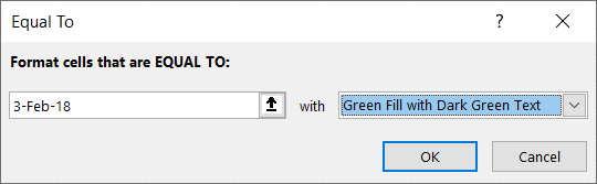
Repeat the same for Green color by creating another dummy rule.


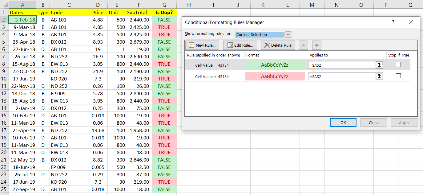
Go to menu item: Home > Conditional Formatting > Manage Rules, you should able to see something as follows:

 
Now, let's try to edit the rules. We can do so by selecting the rule and then click on the " Edit Rule" button.

You should see a dialog exactly like below:


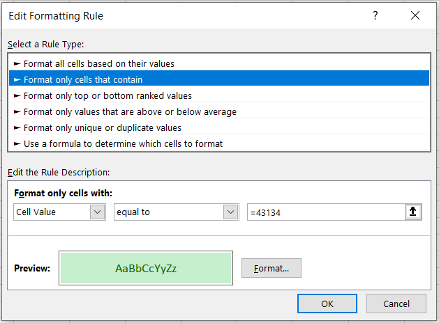
Since the column G already has the values returned as TRUE and FALSE to represent whether the row is duplicate. We will reuse this column and put it into the formula.

So, now let's modify it by selecting " Use a formula to determine which cells to format" from Rule Type, and enter the formula:

=$G2=FALSE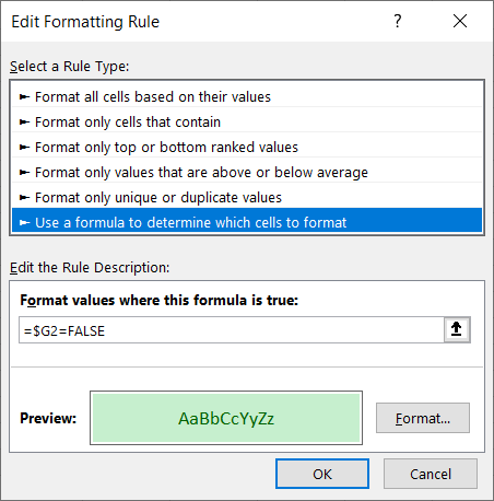

Do remember to change the Applies to, so that we can set the same rule across the selected range. In this case, we can put value:

=$A$2:$F$5000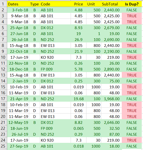

NOTE: You probably need to adjust the end cell (for the example above $5000) in case the list is getting larger and larger. So, try to keep the end cell within a good threshold.

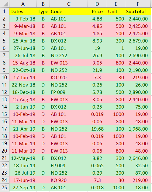
Now, let's modify the Red color rule, by doing the same setting but with formula below:

=$G2=TRUE

And do remember to update the Applies to range as well.

The result is shown as follows:


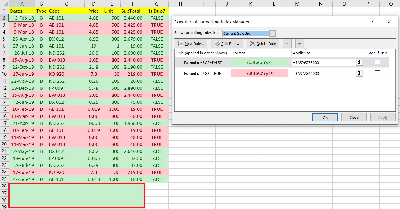
You may already discover that there are empty rows being highlighted with green color. That is because we are applied the rules across the whole columns from $A$2 to $F$5000.

To resolve this issue, we could either:

a) Change the Applied to range, from Let's say:

=$A$2:$F$5000

to:

=$A$2:$F$25

b) OR apply these formulas instead:

For Green rule, use:

=AND($G2=FALSE,$G2<>"")

For Red rule, use:

=AND($G2=TRUE,$G2<>"")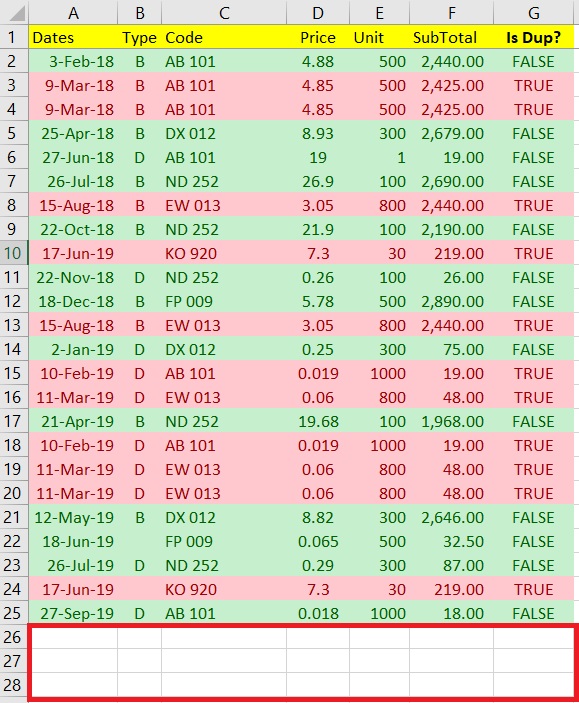

As of now, it looks pretty well a good job for us.


But what if the column G doesn't exist. Can we still highlight the rows which are duplicates?

II ) With Conditional Formatting - Method 2

So, now let's delete the whole column G, you would see that the sheet now is back to blank color while the Conditional Formatting rules still remain.


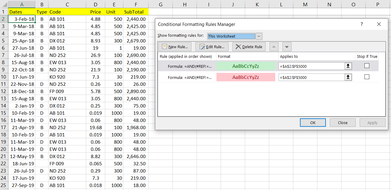
Do note that now there is an #REF! error in the formula in the rules since the reference column G was being deleted.

To make the highlighting can happen again, we need to edit the rule's formula to:

For Green rule, use:

=AND(COUNTIFS($A$2:$A$5000,""&$A2,$B$2:$B$5000,""&$B2,$C$2:$C$5000,""&$C2,$D$2:$D$5000,""&$D2,$E$2:$E$5000,""&$E2,$F$2:$F$5000,""&$F2)=1,$A2&$B2&$C2&$D2&$E2&$F2<>"")

For Red rule, use:

=AND(COUNTIFS($A$2:$A$5000,""&$A2,$B$2:$B$5000,""&$B2,$C$2:$C$5000,""&$C2,$D$2:$D$5000,""&$D2,$E$2:$E$5000,""&$E2,$F$2:$F$5000,""&$F2)>1,$A2&$B2&$C2&$D2&$E2&$F2<>"")

This will produce the result as follows:


NOTE: It would be good to specify the range instead of selecting the whole column, for example:

$A$2:$F$5000 vs $A:$F implementation and some considerations:

• The full column selection will need more computing power. Sometimes, it may hang your Excel.
• The range selection will need less computing power, but you probably need to adjust the end cell (for this article's example, we are using range: $5000) in case the list getting larger and larger. So, try to keep the end cell within a good threshold.

BONUS!!
There is a lot of fun as to what Conditional Formatting can do with formulas, here is an article at Exceljet.net that provide a couple of examples where it can be done.

3. Keep only One Row (De-duping)

There are a couple of ways we can do the de-duping in Excel.

I ) With Wizard

In order to do that, we can follow the steps.

First, select the whole columns from A to F. And then click on menu: Data > Data Tools > Remove Duplicates.

A dialog like below will appear.


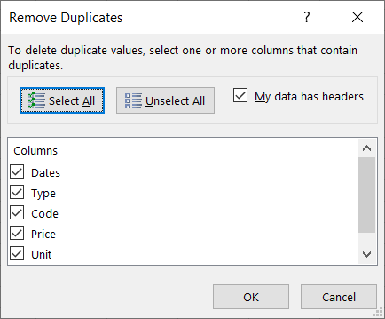
Click OK to proceed.

And now you see in total 6 duplicate rows were removed, and the remaining rows now have become unique rows.


NOTE: We could use the same technique in Part 1: Using Formula to examine the results if it's needed.

II ) With Macro 

In order to do that, we could run Macro below:

Sub test()
    Dim ws As Worksheet
    Set ws = Sheets("Sheet1")
    Call Dedup(ws)
End Sub

Sub Dedup(ws As Worksheet)
    ws.Range("$A2:$F$5000").RemoveDuplicates Columns:=Array(1, 2, 3, 4, 5, 6), Header:=xlYes
End Sub

The RemoveDuplicates function is a call to remove the duplicates from the sheet.

NOTE: We also often call the Macro as VBA Programming as well.

4. Keep only Duplicate Rows

Just in case there is a scenario where we would like to keep only the duplicate rows in a sheet. We still can make it happen and it's pretty easy to do so.

I ) With Wizard

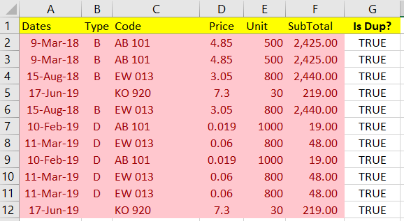
In order to do that, first, let's try to prepare a "Is Dup" column, as what was introduce in Part 1: Using Formula.

It is ok to keep the column G without Conditional Formatting.


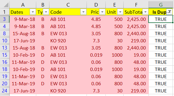
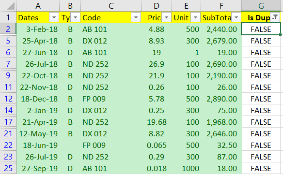
Now, let's try filter the column G with value equals to TRUE, and your list now becomes like this.


Now, click on menu File > Info > Check for Issues > Inspect Document.

A dialog will appear.


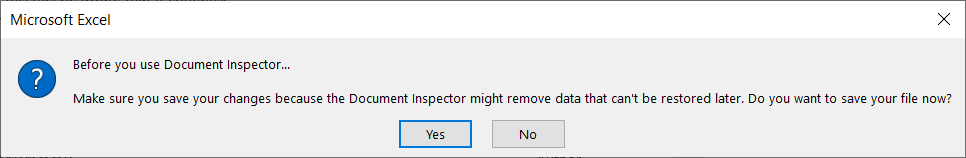
You can click either Yes or No to proceed.

Now, a Document Inspector dialog has appeared. Try unchecking all the options except for " Hidden Rows and Columns".


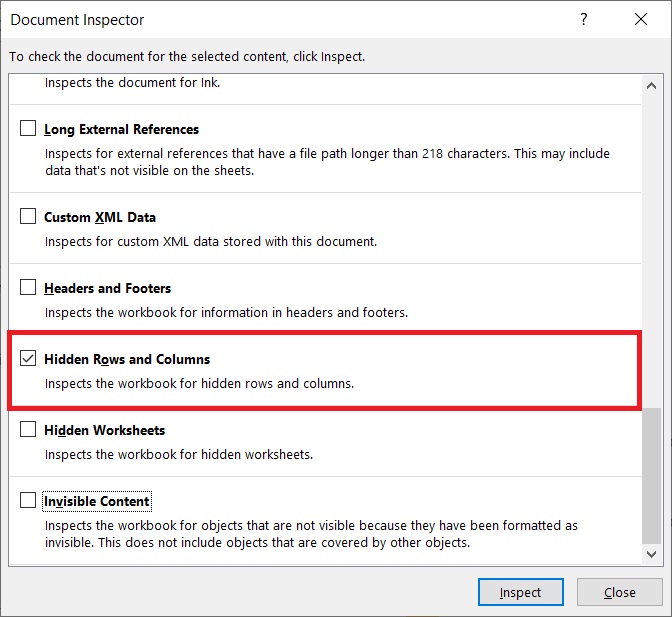
Click Inspect to proceed.
 

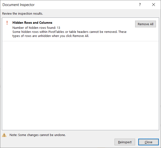
The wizard will tell you the summary of how many rows or columns are affected. Then we can proceed by clicking the " Remove All" button.

Once this is done, exit the dialog and go back to the Sheet.

Now, try to remove the filter on column G and you can see only duplicate rows have remained.


II ) With Macro

We probably can do something similar to the method above but now we do that using Macro.

In case there is already a column G to identify the duplicate rows, it would be pretty much easier for us by running codes below:

Sub test()
    With Application
        .EnableEvents = False
        .ScreenUpdating = False
        .DisplayAlerts = False
    End With
    
    Dim ws As Worksheet
    Set ws = Sheets("Sheet1")
    
    Call ApplyFilter(ws, "G", True)
    Call RemoveHiddenRows(ws)
    Call RemoveFilter(ws)
    
    With Application
        .EnableEvents = True
        .ScreenUpdating = True
        .DisplayAlerts = True
    End With
End Sub


Sub ApplyFilter(ws As Worksheet, Col As String, Value As Variant, Optional rng As String = "A1")
    ColIndex = Range(Col & 1).Column
    ws.Range(rng).AutoFilter Field:=ColIndex, Criteria1:=Value
End Sub


Sub RemoveFilter(ws As Worksheet, Optional rng As String = "A1")
    ws.Range(rng).AutoFilter
End Sub


Sub RemoveHiddenRows(ws As Worksheet, Optional rng As String = "A2")
    Dim r As Range, Row As Range, LastRow As Integer
    Set r = ws.Range(rng)
    LastRow = ws.UsedRange.Rows(ws.UsedRange.Rows.Count).Row
   
    Do Until r.Row > LastRow
        If r.EntireRow.Hidden = True Then
            If Row Is Nothing Then
                Set Row = r.EntireRow
            Else
                Set Row = Union(Row, r.EntireRow)
            End If
        End If
        Set r = r.Offset(1, 0)
    Loop
    If Not Row Is Nothing Then
        Row.Delete
    End If
End Sub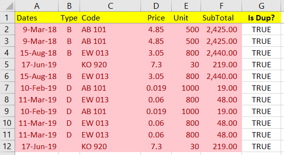

After you run the codes, you will get the result as follows:


It looks like the same as the one we run with the wizard.

In case column G is not available, we probably can use Macro to create it and remove it once the process is done.

Sub CreateFormula(ws As Worksheet, Col As String)
    Dim idx As Integer, LastRow As Integer, formulaStr As String
    
    idx = Range(Col & "1").Column
    For i = 1 To idx
        formulaStr = IIf(i = idx, "", ",") & "C[-" & i & "],""""&RC[-" & i & "]" & formulaStr
    Next
    LastRow = ws.UsedRange.Rows(ws.UsedRange.Rows.Count).Row
    
    ws.Range(Col & "2:" & Col & LastRow).FormulaR1C1 = "=COUNTIFS(" & formulaStr & ")>1"
End Sub

Sub DeleteColumn(ws As Worksheet, Col As String)
    ws.Columns(Col).EntireColumn.Delete
End Sub

To call the functions:

Sub test2()
    With Application
        .EnableEvents = False
        .ScreenUpdating = False
        .DisplayAlerts = False
    End With
    
    Dim ws As Worksheet
    Set ws = Sheets("Sheet1")
    
    Call CreateFormula(ws, "G")
    Call ApplyFilter(ws, "G", True)
    Call RemoveHiddenRows(ws)
    Call RemoveFilter(ws)
    Call DeleteColumn(ws, "G")
    
    With Application
        .EnableEvents = True
        .ScreenUpdating = True
        .DisplayAlerts = True
    End With
End Sub

After you made that changes and run the Macro, you will get the result as follows:


5. Delete the Duplicate Rows

To delete the duplicate rows is actually the opposite result of Part 4: Keep only Duplicate Rows.

I ) With Wizard

In order to do that, first, let's try to prepare a "Is Dup" column, as what was introduce in Part 1: Using Formula.

It is ok to keep the column G without Conditional Formatting.



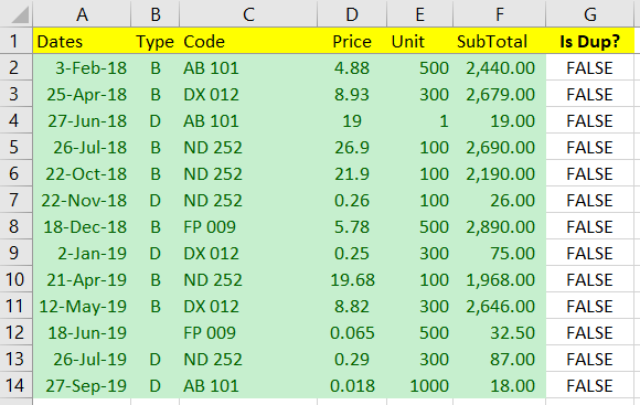
Now, let's try filter the column G with value equals FALSE, and your list now becomes like this.


Now, click on menu File > Info > Check for Issues > Inspect Document to open the Document Inspector dialog and proceed to remove the hidden rows and columns.



Once this is done, exit the dialog and go back to the Sheet.

Now, try to remove the filter on column G and you can see only unique rows have remained.


II ) With Macro

Since we have already written the Macro in Part 4: Keep only Duplicate Rows, we can re-use the same codes with different parameters.

In case there is already a column G to identify the duplicate rows, it would be pretty much easier for us by running codes below:

Sub test()
    With Application
        .EnableEvents = False
        .ScreenUpdating = False
        .DisplayAlerts = False
    End With
    
    Dim ws As Worksheet
    Set ws = Sheets("Sheet1")
    
    Call ApplyFilter(ws, "G", False)
    Call RemoveHiddenRows(ws)
    Call RemoveFilter(ws)
    
    With Application
        .EnableEvents = True
        .ScreenUpdating = True
        .DisplayAlerts = True
    End With
End Sub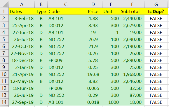

In case column G is not available, we simply modify the Test2 procedure and test it.

Sub test2()
    With Application
        .EnableEvents = False
        .ScreenUpdating = False
        .DisplayAlerts = False
    End With
    
    Dim ws As Worksheet
    Set ws = Sheets("Sheet1")
    
    Call CreateFormula(ws, "G")
    Call ApplyFilter(ws, "G", False)
    Call RemoveHiddenRows(ws)
    Call RemoveFilter(ws)
    Call DeleteColumn(ws, "G")
    
    With Application
        .EnableEvents = True
        .ScreenUpdating = True
        .DisplayAlerts = True
    End With
End Sub

You should able to get the desired result as well.


6. Move the Duplicate or Unique Rows to Another Sheet

In order to move the duplicate rows to another sheet, we would need to write Macro codes to do that.

For this task, we will need to introduce some more functions/ procedures:

Function CreateSheet(wb As Workbook, wsName As String) As Worksheet
    Dim ws_target As Worksheet
    Set ws_target = wb.Worksheets.Add(After:=wb.Worksheets(wb.Worksheets.Count))
    ws_target.Name = "Output"
    Set CreateSheet = ws_target
End Function


Function DeleteSheet(wb As Workbook, wsName As String) As Boolean
    Dim Sheet As Worksheet
   
    For Each Sheet In wb.Worksheets
        If UCase(Sheet.Name) = UCase(wsName) Then
            Application.DisplayAlerts = False
            Sheet.Delete
            Application.DisplayAlerts = True
            DeleteSheet = True
            Exit Function
        End If
    Next
    DeleteSheet = False
End Function


Sub MoveFilteredRows(ws_source As Worksheet, ws_target As Worksheet)
    ws_source.UsedRange.SpecialCells(xlCellTypeVisible).Copy
    With ws_target.Cells(1, 1)
        .PasteSpecial
        .PasteSpecial xlPasteColumnWidths
        .PasteSpecial xlPasteValues
        .PasteSpecial xlPasteFormats
    End With
    Application.CutCopyMode = False
    ws_target.Cells(1, 1).Select
End Sub


Sub ClearContent(ws As Worksheet, Col As String)
    ws.Columns(Col & ":" & Col).ClearContents
End Sub

To test the codes, we would need test3 procedure:

Sub test3()
    With Application
        .EnableEvents = False
        .ScreenUpdating = False
        .DisplayAlerts = False
    End With
   
    Dim wb_target As Workbook
    Dim ws_source As Worksheet, ws_target As Worksheet
   
    Set ws_source = Sheets("Sheet1")
    Set wb_target = ws_source.Parent
   
    Call DeleteSheet(wb_target, "Output")
    Set ws_target = CreateSheet(wb_target, "Output")
   
    Call CreateFormula(ws_source, "G")
    Call ApplyFilter(ws_source, "G", True)
    Call ClearContent(ws_source, "G")
    Call MoveFilteredRows(ws_source, ws_target)
    Call RemoveFilter(ws_source)
    Call DeleteColumn(ws_source, "G")
   
    With Application
        .EnableEvents = True
        .ScreenUpdating = True
        .DisplayAlerts = True
    End With
End Sub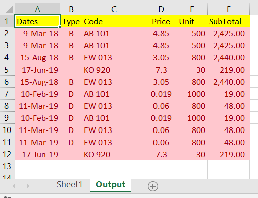

Once you run the codes above, you can see a new sheet named as "Output" being generated with all duplicate rows.


Well, you may ask what if I want to export the unique rows to "Output" sheet instead? I guess you already know the answer by changing the filter value:

Sub test4()
    With Application
        .EnableEvents = False
        .ScreenUpdating = False
        .DisplayAlerts = False
    End With
   
    Dim wb_target As Workbook
    Dim ws_source As Worksheet, ws_target As Worksheet
   
    Set ws_source = Sheets("Sheet1")
    Set wb_target = ws_source.Parent
   
    Call DeleteSheet(wb_target, "Output")
    Set ws_target = CreateSheet(wb_target, "Output")
   
    Call CreateFormula(ws_source, "G")
    Call ApplyFilter(ws_source, "G", False)
    Call ClearContent(ws_source, "G")
    Call MoveFilteredRows(ws_source, ws_target)
    Call RemoveFilter(ws_source)
    Call DeleteColumn(ws_source, "G")
   
    With Application
        .EnableEvents = True
        .ScreenUpdating = True
        .DisplayAlerts = True
    End With
End Sub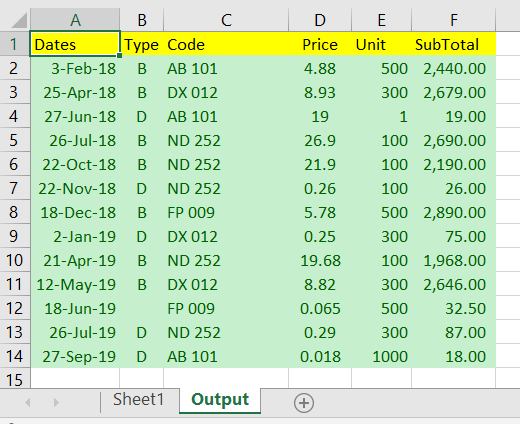

---

Short Summary

I guess I have addressed most of the popular issues dealing with duplicate rows in Excel. If you still have any issues that cannot be resolved by applying the above methods, or if you have any suggestions to improve this article, do try to reach me either publicly or privately.

Take care and cheers.