Creating a legend for conditional formatting in Excel 2016 and a hyperlink to that legend

I thought the spreadsheet I created was not only fairly cool, but since it had a bunch of different conditional formatting (read more about conditional formatting in my article here ) that highlighted different rows depending on the values entered, explained itself fairly well.  I was wrong about this, although it took an oblique comment in order for me to find that out.  The spreadsheet I created just tracked membership for a relatively small group (less than a thousand).  I had created about 25 different rules that determined what font and background each row was assigned (those were the conditional formatting rules).  A colleague asked me to go over how it worked with him because he was a little confused.  This guy is a former VP of Pepsico, so no slouch.  It was then that I realized I had to include some better instructions.

I decided that one way to make this clearer was to incorporate a legend.  As I usually do, I searched both EE and the rest of the internet for the best ways to make this legend.  The result of my searches came down to "Take a screenshot of the rules manager."  Which works, but the result is not as useful as you might think.

This screenshot method required me to take successive screenshots of the rules (since a screenshot can only get 4-5 at a time, I needed 5 screenshots.).  Each screenshot I pasted into the spreadsheet.  The process went as follows:

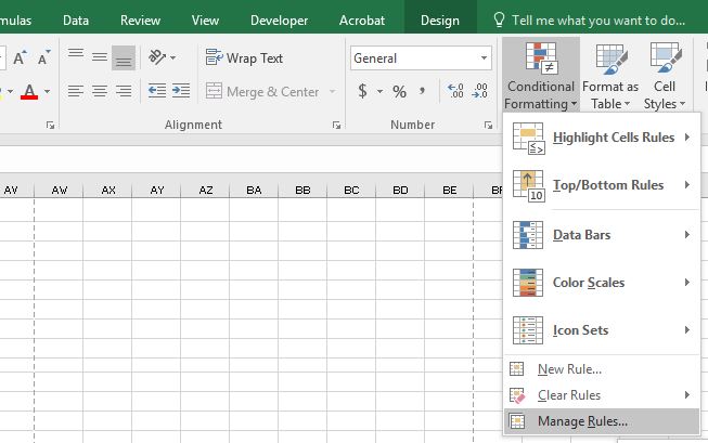
I went to the Conditional Formatting dropdown and selected "Manage Rules"

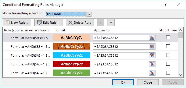
After selecting Manage rules, the conditional Formatting Rules Manager appears

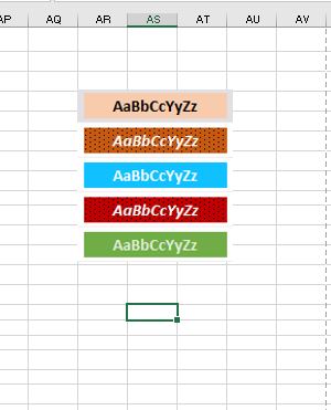
Use any screenshot tool (I used the Windows 10 built-in snipping tool) to capture and either copy or save the selection.  Then either insert it or paste it into your spreadsheet.  The result will be similar to the one below.

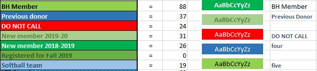
Why not just do it this way?  The answer was relatively easy for me, first of all, the function of a legend should be explanatory, this really wasn't.  Although the formatting that would result if the rule was true is there, it just says "AaBbCcYyZz" for each and every rule.  To make it make any sense you would then have to match the formatting to what it means - no easy task if you have a lot of rules.

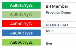
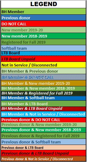
Here is how it looks with a brief explanation next to it:

So after trying that suggestion, I had an overnight epiphany, use the paintbrush tool to copy the rules and change the value that triggers each rule.  This was by no means easy.  To make the Legend clearer, I deleted all rules except the one I needed, which meant doing each part of the legend separately.  

Although the result was more than satisfactory, it takes more than a couple of steps to do it, depending on the number of conditional formatting rules you have.  The final result looked like this:

As compared to the cut and paste method:

The task went as follows:

The first step was to create the text that I wanted each legend section to have.  I decided that having dynamic text would be best (change it in one place and it changes in the other).  I create a basic formula that pointed to the text I wanted (=<target text>) and the target text was the title of a column.  So the cell that says "BH Member" has an underlying formula of "=Table13[[#Headers],[BH Member]]" (without the quotes) and so forth on down the list.  The items that have an ampersand (&) in them have a slightly different formula, such as "=CONCATENATE($AE$2," & ",AE3)" (without the quotes).

Once all the names have been created, I went on to the next step.  The second step was to use the paintbrush tool to copy all the conditional formatting on to each legend cell.  I did this one at a time, otherwise, it became rather confusing as to which rules were being applied to which cells.  

1. Copy, using the Paintbrush Tool, the formatting from inside the table to the first legend cell, labeled "BH Member."
2. Delete all the rules except the one that is applied to this legend entry
3. Edit the rule so that it will trigger when it is equal to the text in the cell (if it equals itself)
4. Then apply the rule and click okay

I repeated 1-4 for each legend entry.

The end result was the legend I posted above (I entered the word LEGEND in the first cell).

The third and final step was to create a hyperlink at the beginning of the document/spreadsheet that would take you directly to the legend.  There were several smaller steps to do this.

1. Name the range from where the word LEGEND is to the last legend piece, "Legend"
   1. Highlight the range
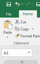
   2. in the range name box (in the picture it reads "A1" type the name Legend to name the range or right-click and select define name.
   3. Now that the range has been named, it is easier to create a hyperlink to that legend.  Type something like "go to Legend" in a cell near the home cell of your worksheet.  I highlighted the cell to make it stand out.  
      1. Right-click on the cell and select hyperlink.
      2. The hyperlink dialogue will appear.  Select "Place in this Document" on the side and the defined name "Legend"
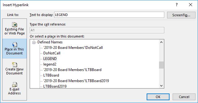
      3. Click OK when you are done
      4. You may need to get rid of underlining
      5. When I was done it looked like this:

That was how I created the spreadsheet with a real legend.

I hope you found this article useful. You are encouraged to ask questions, report any bugs or make any other comments about it below.

Note: If you need further "Support" about this topic, please consider using the Ask a Question feature of Experts Exchange. I monitor questions asked and would be pleased to provide any additional support required in questions asked in this manner, along with other EE experts...

Please do not forget to press the "Thumb's Up" button if you think this article was helpful and valuable for EE members.

It also provides me with positive feedback. Thank you!