Duplicating relative conditional formatting over a large range of cells in Excel
Hello,
In Excel (2007), how can a range of cells with Conditional Formatting (CF) be copy/pasted into another range of cells in a way that RELATIVE CF is transferred?
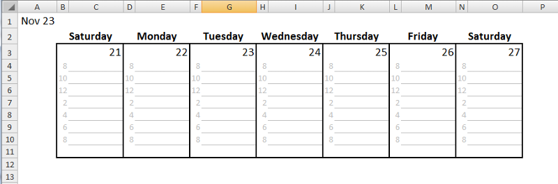
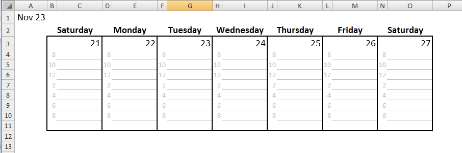
As an example, suppose you want to create a full-year calendar beginning with the current week as shown in Fig. A,
 in which dates are calculated as shown in Fig. B
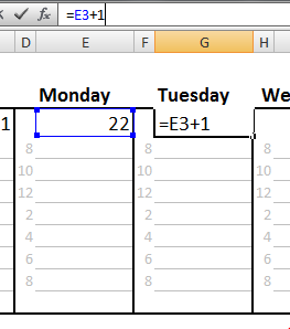 (except Sundays which are calculate from the previous Saturday)
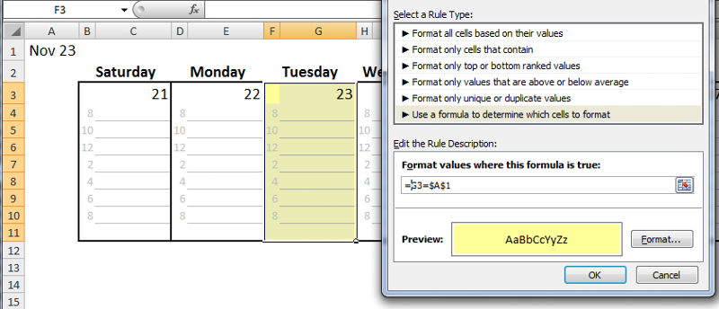
Also, suppose you want CF applied so that the current day will automatically change to a yellow fill. This can be done by setting a separate cell (like A1) to
=TODAY()
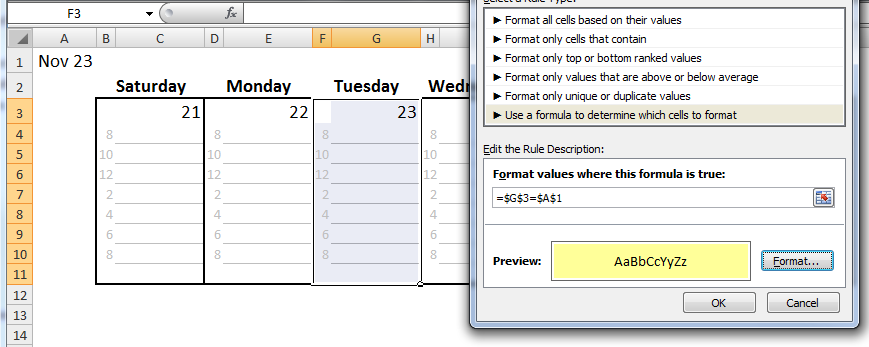
and then applying CF as shown in Fig. C
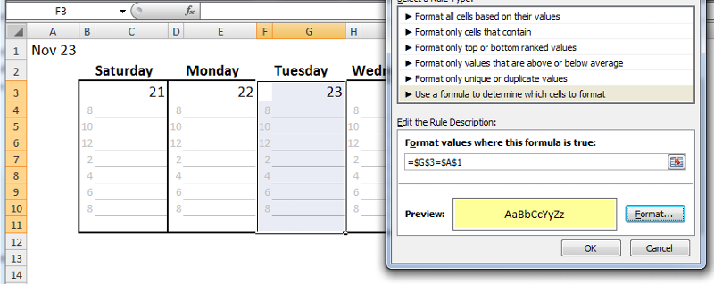 which produces the result shown in Fig. D

Now, the question is how can that same CF be applied to the other days in the calendar? If the CF day (the 23rd) is simply copy/pasted to another day (the 24th), you end up with the situation shown in Fig. E
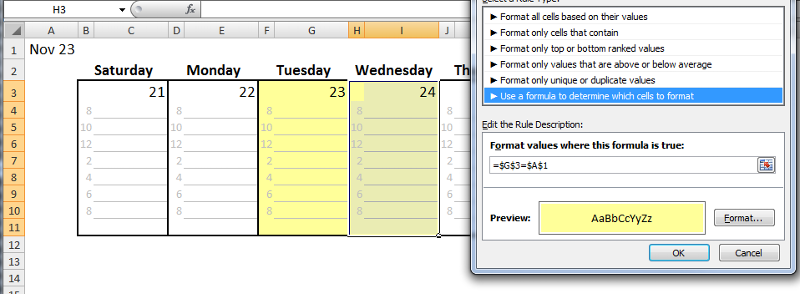 where, because the original reference in the 23rd is absolute ($G$3), now the 24th lights up also. Thus, although the relative formula for the date is OK (showing the value, 24), the CF for all the cells in the range comprising the 24th is actually tied to the 23rd.
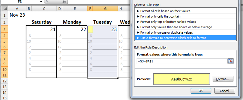
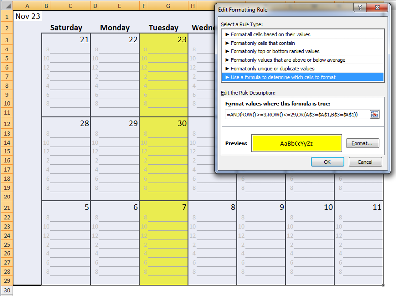
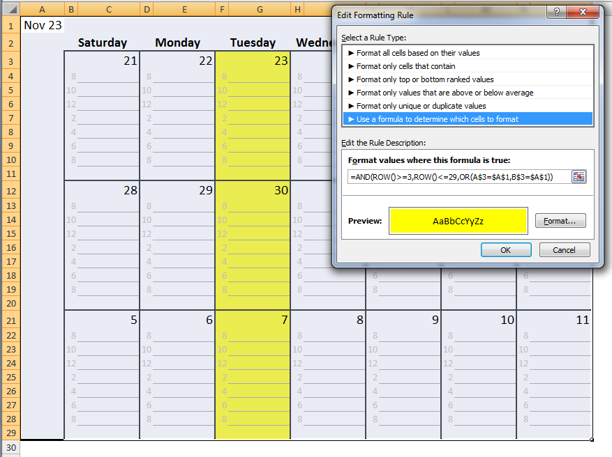
Alternatively, if you go back and change the initial CF to a relative reference (Fig. F),
 then it only formats the upper-left cell in the range (Fig. G).
 Therefore, aside from doing it by hand, how can something the size of this calendar be CF, let alone, something many times larger?
Thanks
In Excel (2007), how can a range of cells with Conditional Formatting (CF) be copy/pasted into another range of cells in a way that RELATIVE CF is transferred?
As an example, suppose you want to create a full-year calendar beginning with the current week as shown in Fig. A,
 in which dates are calculated as shown in Fig. B(except Sundays which are calculate from the previous Saturday)
Also, suppose you want CF applied so that the current day will automatically change to a yellow fill. This can be done by setting a separate cell (like A1) to
=TODAY()
and then applying CF as shown in Fig. C
 which produces the result shown in Fig. D
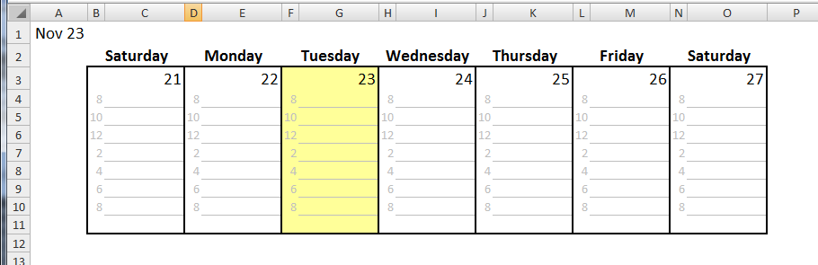
Now, the question is how can that same CF be applied to the other days in the calendar? If the CF day (the 23rd) is simply copy/pasted to another day (the 24th), you end up with the situation shown in Fig. E
 where, because the original reference in the 23rd is absolute ($G$3), now the 24th lights up also. Thus, although the relative formula for the date is OK (showing the value, 24), the CF for all the cells in the range comprising the 24th is actually tied to the 23rd.
Alternatively, if you go back and change the initial CF to a relative reference (Fig. F),
 then it only formats the upper-left cell in the range (Fig. G).
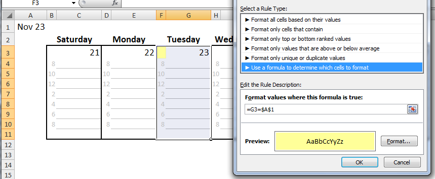 Therefore, aside from doing it by hand, how can something the size of this calendar be CF, let alone, something many times larger?
Thanks
Putting both G and H should make it work for the offset. (might need F and G, I didn't test yet).
Okay, I tested it and it's working just fine. Alternatively you could select your whole sheet and use this formula
=and(row()>3,row()<12,OR(A
=and(row()>3,row()<12,OR(A
Steve,
One trick you may like:
1) Click anywhere in a cell reference in a formula by in the formula bar (such as between the D and the 1 in the formula =D1+G13*H1
2) Click the F4 key repeatedly to toggle between the four possible absolute and relative address modes like $D$1, D$1, $D1, D1, ...
If you select a character between two cell references (such as + or :) then the F4 toggles both the cell before and after through the four absolute and relative possibilities.
This same trick with the F4 also works in the Conditional Formatting dialog.
Brad
ASKER
Thanks for the responses.
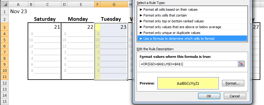
>>Try =Or(G$3=$A$1,H$3=$A$1)
Pasting this in CF for the 23rd (F3:G11) results in this:
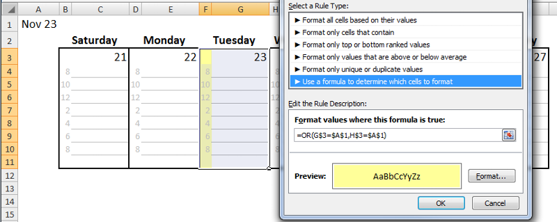
In which only column F is yellow.
>>Try =Or(G$3=$A$1,H$3=$A$1)
Pasting this in CF for the 23rd (F3:G11) results in this:
In which only column F is yellow.
Use =Or(F$3=$A$1,G$3=$A$1)
My big formula has an error. Apply this to the whole sheet
=and(row()>=3,row()<=11,OR
=and(row()>=3,row()<=11,OR
ASKER
>>My big formula has an error. Apply this to the whole sheet
=and(row()>=3,row()<=11,OR
Tommy, you are getting closer! It works great for any day this week but when I copy/pasted the week down to form next week, it no longer worked. It would be nice to have a "template" to just paste at the bottom to form a new week but I don't know if that is possible.
I also tried, after making a third week, changing the bottom row term from,
row()<=11, to row()<=29,
i.e. =and(row()>=3,row()<=29,OR
to match the new bottom row, but with A1 = Nov 23, that gave me this:
 It was the same for A1 = to any day of this week (e.g. A1 = Nov 25 highlighted 11/25, 12/2 and 12/9). However, setting A1 to any other date (11/28-12/11) produced no yellow anywhere.
Ah, you are going down rows. This will take a modulo operator, give me a minute.
Okay, use this condition for the whole sheet.
=OFFSET($A$1,9*FLOOR((ROW(
=OFFSET($A$1,9*FLOOR((ROW(
ASKER
A what-ulo operator?
I thought I was going to use modulo (the mod function). mod is a good way to make a lot of numbers transform into a few numbers as are integer division and rounding. I ended up using floor. Anyway, as long as you leave your calendar set up like it is this will work
=OFFSET($A$1,9*FLOOR((ROW(
Note, the 9s are for the height of the day. If you make the days taller, make the 9s bigger
=OFFSET($A$1,9*FLOOR((ROW(
Note, the 9s are for the height of the day. If you make the days taller, make the 9s bigger
The 2s in 2*floor(column()/2 are for the width of the days.
The only other thing to worry about is the shifting, this is a bit more complicated, but if you leave the number of blank rows above and to the left of the calendar as they are it should always work. If you do end up wanting help adjusting this again later, just click on 'ask a related question' and it will email me and I can help.
The only other thing to worry about is the shifting, this is a bit more complicated, but if you leave the number of blank rows above and to the left of the calendar as they are it should always work. If you do end up wanting help adjusting this again later, just click on 'ask a related question' and it will email me and I can help.
SOLUTION
membership
This solution is only available to members.
To access this solution, you must be a member of Experts Exchange.
Sample file attached using MOD function for Conditional Formatting
CalendarQ26635378.xlsx
CalendarQ26635378.xlsx
ASKER
>>One trick you may like:....Click the F4 key repeatedly to toggle between the four possible absolute and relative address modes
Thanks Brad. That's one trick that I have known for a while and it is a big time saver. However, don't let my knowing that one prevent you from posting others anytime you think of them because you have enhanced my Excel-ability many times in the past and I am looking forward to you doing the same many more times in the future!
Thanks Brad. That's one trick that I have known for a while and it is a big time saver. However, don't let my knowing that one prevent you from posting others anytime you think of them because you have enhanced my Excel-ability many times in the past and I am looking forward to you doing the same many more times in the future!
ASKER
Thanks form the responses.
>>=OFFSET(B3,-MOD(ROW()-3,
Brad, I downloaded your file and it obviously works but since I have several places to apply this type of Conditional Formatting (CF) function and not having used MOD before or OFFSET this way, I have spent some time trying to understand why/how it works and I'm not quite there:
1) It appears that you can copy/paste a single or range of cells and preserve the CF as long as the copy range and paste range are both within the original range (OR = B3:O48) to which the CF was applied. Is that correct?
2) If some range within the OR is copied and then pasted outside of the OR, the CF no longer applies or at least is not correct. If that is true, then it's clear that trying to determine the final range at the beginning of the project is important. However, knowing that is not always possible, is there some way, or what is the best way to enlarge the OR after the CF has been applied?
3) Inserting and/or deleting rows/columns once the CF is applied also messes up the OR -- particularly downstream (down and right) from the point of insertion. If that is true...(same questions as above).
4) Regarding the actual CF formula, can you get me straightened out on how it works? Fig. 1 shows your CF formula and the file you posted with modifications to show only two weeks. The date in A1 has been set to Nov 10 and several unneeded rows in the first week have been hidden. Also, the offset origin for your formula is green and the gray numbering in Row 2 and Column A are relative to that origin.
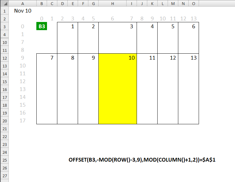
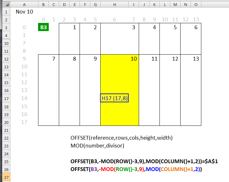
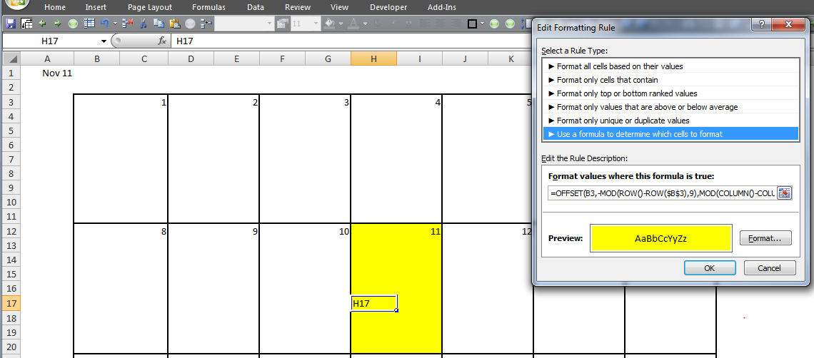
Fig. 2 shows an arbitrarily-selected cell (H17) inside Nov 10 with its numeric (absolute) coords. There's also some other info to help me stay on track.
In Fig. 3, I changed the formula to an IF form (minus the equal sign) with the letter "Y" to indicate if it is true. (Can I do that? Probably not since where I'm going with this does not turn out well...) I also substituted the ROW() and COLUMN() values as they would be in cell H17.
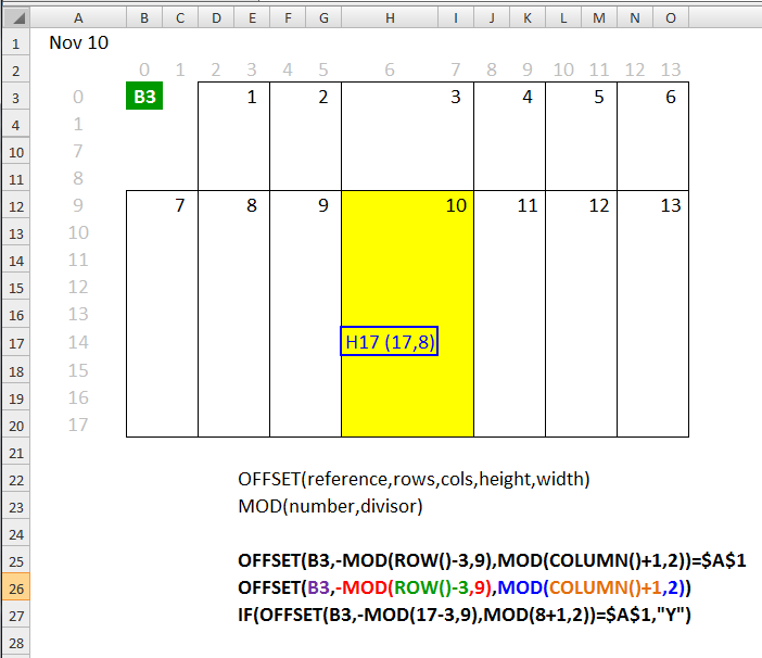
Finally, I simplified to get the results shown in Fig. 4.

Those last three IF formulas all return #REF! when equal signs are inserted so, as I said earlier, I know I did something wrong. However, I think I understand the idea, namely, to get back to the date in the upper-right corner -- from any cell in the range representing a single day -- in order to see if it matches A1 (Fig. 5).
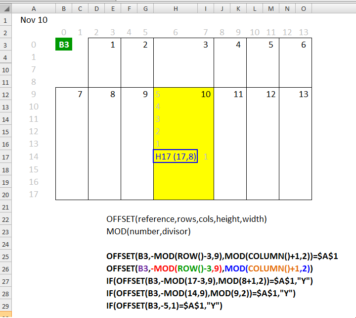
The main thing I don't understand is how you get the resulting OFFSET coords (-5, 1 in this case), to measure from H17 since your OFFSET formula specifies B3 as the origin.
Thanks
"A person who has never made a mistake is a person who has never tried anything new." ~Albert Einstein
>>=OFFSET(B3,-MOD(ROW()-3,
Brad, I downloaded your file and it obviously works but since I have several places to apply this type of Conditional Formatting (CF) function and not having used MOD before or OFFSET this way, I have spent some time trying to understand why/how it works and I'm not quite there:
1) It appears that you can copy/paste a single or range of cells and preserve the CF as long as the copy range and paste range are both within the original range (OR = B3:O48) to which the CF was applied. Is that correct?
2) If some range within the OR is copied and then pasted outside of the OR, the CF no longer applies or at least is not correct. If that is true, then it's clear that trying to determine the final range at the beginning of the project is important. However, knowing that is not always possible, is there some way, or what is the best way to enlarge the OR after the CF has been applied?
3) Inserting and/or deleting rows/columns once the CF is applied also messes up the OR -- particularly downstream (down and right) from the point of insertion. If that is true...(same questions as above).
4) Regarding the actual CF formula, can you get me straightened out on how it works? Fig. 1 shows your CF formula and the file you posted with modifications to show only two weeks. The date in A1 has been set to Nov 10 and several unneeded rows in the first week have been hidden. Also, the offset origin for your formula is green and the gray numbering in Row 2 and Column A are relative to that origin.
Fig. 2 shows an arbitrarily-selected cell (H17) inside Nov 10 with its numeric (absolute) coords. There's also some other info to help me stay on track.
In Fig. 3, I changed the formula to an IF form (minus the equal sign) with the letter "Y" to indicate if it is true. (Can I do that? Probably not since where I'm going with this does not turn out well...) I also substituted the ROW() and COLUMN() values as they would be in cell H17.
Finally, I simplified to get the results shown in Fig. 4.
Those last three IF formulas all return #REF! when equal signs are inserted so, as I said earlier, I know I did something wrong. However, I think I understand the idea, namely, to get back to the date in the upper-right corner -- from any cell in the range representing a single day -- in order to see if it matches A1 (Fig. 5).
The main thing I don't understand is how you get the resulting OFFSET coords (-5, 1 in this case), to measure from H17 since your OFFSET formula specifies B3 as the origin.
Thanks
"A person who has never made a mistake is a person who has never tried anything new." ~Albert Einstein
Just take one you can apply to the whole sheet. If you want it to ignore certain rows do something like this
=AND(OFFSET($A$1,9*FLOOR((
So it will only format rows > row 3 and columns < column 60
=AND(OFFSET($A$1,9*FLOOR((
So it will only format rows > row 3 and columns < column 60
SOLUTION
membership
This solution is only available to members.
To access this solution, you must be a member of Experts Exchange.
ASKER
Brad, thanks a bunch for the detailed explanation.
Before commenting or asking other questions, I need to get this resolved because it may be at the heart of the issue I posted earlier.
In your explanation, you said:
>>If you select cell H17 and look at the Conditional Formatting formula in that cell, you will find that it has changed to:
=OFFSET(H17,-MOD(ROW()-ROW
I am obviously doing something wrong because when I look at the CF formula for cell H17, I see this:
=OFFSET(B3,-MOD(ROW()-ROW(
This is from the file you just attached but B3 is the reference for mine as well (see above).
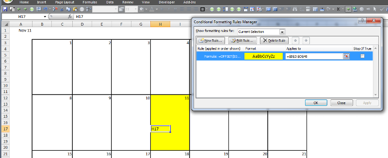
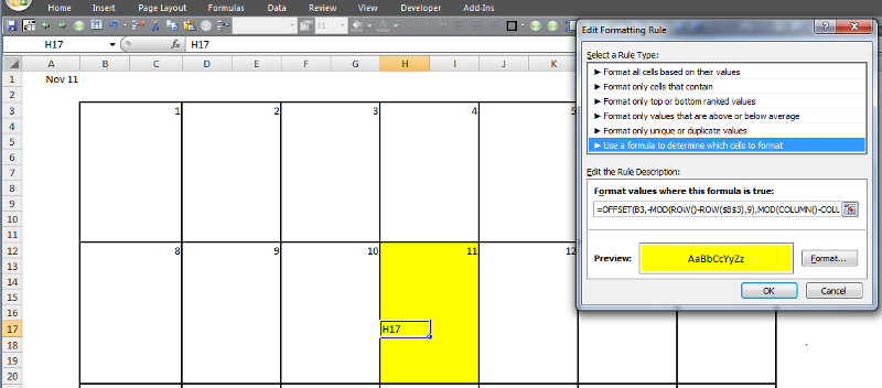
Maybe we are talking about/looking at different things. Included below, are some live action shots of me checking the CF for cell H17. (I would post the video also if EE allowed it. However, you may be able to view it tomorrow on ESPN's weekend highlights!) :)
To check the CF, I did the following:
1) clicked cell H17
2) clicked the CF icon on my QAT (Fig. 1) which brought up the
3) Conditional Formatting Rules Manager (Fig. 2) in which I clicked "Edit Rule" which opened the
4) Edit Formatting Rule box (Fig. 3) which shows the formula.
Unless it's too small, you can see that it references B3 as shown above rather than H17. If you can tell me what may be causing that difference, we may have it solved.
Thanks

Before commenting or asking other questions, I need to get this resolved because it may be at the heart of the issue I posted earlier.
In your explanation, you said:
>>If you select cell H17 and look at the Conditional Formatting formula in that cell, you will find that it has changed to:
=OFFSET(H17,-MOD(ROW()-ROW
I am obviously doing something wrong because when I look at the CF formula for cell H17, I see this:
=OFFSET(B3,-MOD(ROW()-ROW(
This is from the file you just attached but B3 is the reference for mine as well (see above).
Maybe we are talking about/looking at different things. Included below, are some live action shots of me checking the CF for cell H17. (I would post the video also if EE allowed it. However, you may be able to view it tomorrow on ESPN's weekend highlights!) :)
To check the CF, I did the following:
1) clicked cell H17
2) clicked the CF icon on my QAT (Fig. 1) which brought up the
3) Conditional Formatting Rules Manager (Fig. 2) in which I clicked "Edit Rule" which opened the
4) Edit Formatting Rule box (Fig. 3) which shows the formula.
Unless it's too small, you can see that it references B3 as shown above rather than H17. If you can tell me what may be causing that difference, we may have it solved.
Thanks

SOLUTION
membership
This solution is only available to members.
To access this solution, you must be a member of Experts Exchange.
ASKER
Brad,
If anyone is silly my friend, it's aint you! I'm the one who feels silly because after all this discussion I'm feeling more confused than ever -- so I went back to something much more basic. Unfortunately, that confused me even more! lol
Please help me with this:
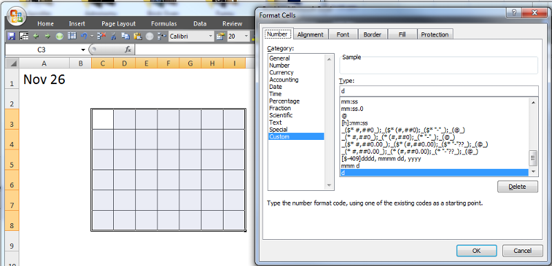
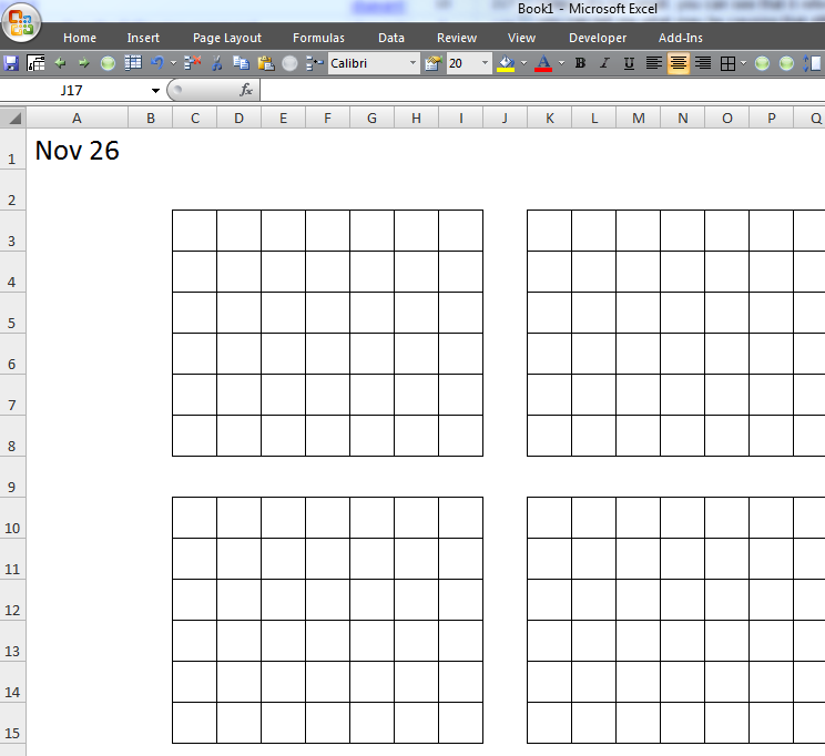
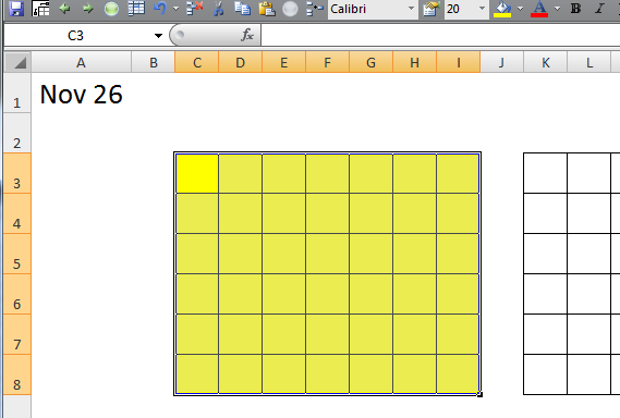
I started anew with a blank sheet and with =NOW() in A1 (formatted as mmm d). I then decided to have just one cell represent each day. I fomatted each cell in this grid to "d" (Fig.1) and made some copies (Fig. 2).
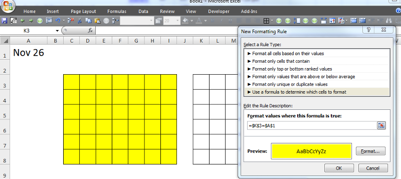
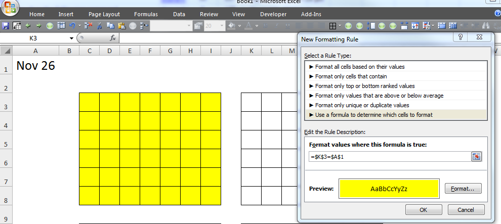
 I then selected the 1st grid (C3:I8) and CF to =$A$1 (Fig. 3)
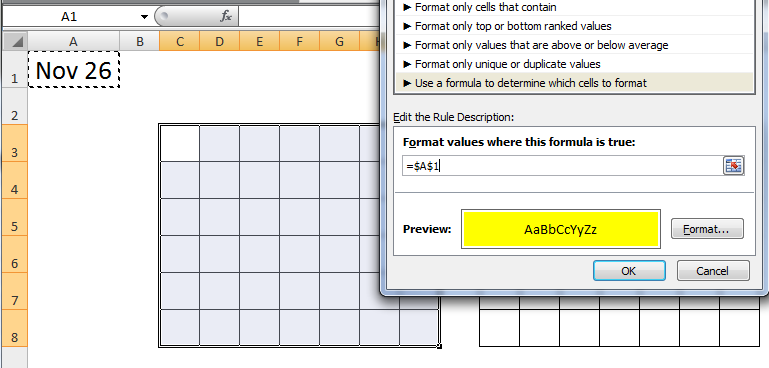 However, with that, as soon as I clicked OK, it immediately changed the whole thing to yellow (Fig. 4) even with no values entered. Why would it do that?
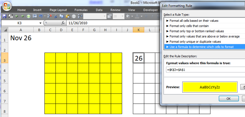
Next, I selected only the 1st cell (K3) in the 2nd grid and entered =$K$3=$A$1 as the CF formula (Fig. 5)
 and just for kicks, I entered 11/26 into that same cell (K3), but to my total surprise, it did not light up (Fig. 6)
I tried some other things in the remaining grids Brad, but I've got myself so confused that I'm going to stop here and hope that you or someone can rescue me. It may just me be but this whole CF process seems quite non-intuitive considering the rules and conventions used with regular formulas and how you can copy/paste them.
Thanks
If anyone is silly my friend, it's aint you! I'm the one who feels silly because after all this discussion I'm feeling more confused than ever -- so I went back to something much more basic. Unfortunately, that confused me even more! lol
Please help me with this:
I started anew with a blank sheet and with =NOW() in A1 (formatted as mmm d). I then decided to have just one cell represent each day. I fomatted each cell in this grid to "d" (Fig.1) and made some copies (Fig. 2).
 I then selected the 1st grid (C3:I8) and CF to =$A$1 (Fig. 3)However, with that, as soon as I clicked OK, it immediately changed the whole thing to yellow (Fig. 4) even with no values entered. Why would it do that?
Next, I selected only the 1st cell (K3) in the 2nd grid and entered =$K$3=$A$1 as the CF formula (Fig. 5)
 and just for kicks, I entered 11/26 into that same cell (K3), but to my total surprise, it did not light up (Fig. 6)
I tried some other things in the remaining grids Brad, but I've got myself so confused that I'm going to stop here and hope that you or someone can rescue me. It may just me be but this whole CF process seems quite non-intuitive considering the rules and conventions used with regular formulas and how you can copy/paste them.
Thanks
ASKER CERTIFIED SOLUTION
membership
This solution is only available to members.
To access this solution, you must be a member of Experts Exchange.
ASKER
Brad, thanks for the the compliment. It means a lot, particularly coming from you.
Also, thanks for backing out with me to the broader view re CF. The understanding and perspective conveyed in your last post will help immensly as I drill back down!
In the mean time however, so that I can move past this snag to which I have been tethered for several days (and if it won't take too much time), would you mind telling me, in specific terms, just how you would CF the two examples in this thread or point out where that's been done?
I trust that the solution will become clear as I spend some time going back through the comments and working through some examples but in the interest of a project I would like to wrap up this weekend, having a "plug & play" solution would be very helpful.
Thanks again
SOLUTION
membership
This solution is only available to members.
To access this solution, you must be a member of Experts Exchange.
ASKER
Thanks a bunch Brad. That's just what I needed!
ASKER
multiple good answers
Using G$3 makes the column relative but the row absolute