Excel - Add up values from a column from multiple workbooks
Hi Excel Experts,
I have multiple Excel Workbooks. (Example attached) Jaggar---Bookstore.zip
Inside of these files you will see a sheet which looks like this: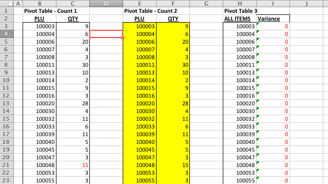
Each file has different numbers (in different order). Here is another workbook screenshot: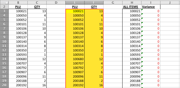
What I need to do is add up all the numbers from the sheet into a single data set. (Only the yellow highlighted part). [Don't pay attention to the other sheets, in the workbook. We are only focusing on the yellow highlighted part). (I know I could use a pivot table, and copy all of the data into a single sheet; but I would prefer to do this using a formula).
Can someone help?
ASKER
Hi Teylyn,
I tried doing it. I put into a new workbook this formula:
However, I get a #N/A when I do that formula.
I tried doing it. I put into a new workbook this formula:
=VLOOKUP(A1,'[Zone 1 - Jag Bookstore.xlsx]Variance'!$E$3:$F$153,2,FALSE)+VLOOKUP(A1,'[Zone 2 - Jag Bookstore.xlsx]Variance'!$E$3:$F$74,2,FALSE)+VLOOKUP(A1,'[Zone 3 - Jag Bookstore.xlsx]Variance'!$E$3:$F$68,2,FALSE)+VLOOKUP(A1,'[Zone 4 - Jag Bookstore.xlsx]Variance'!$E$3:$F$125,2,FALSE)+VLOOKUP(A1,'[Zone 5 - Jag Bookstore.xlsx]Variance'!$E$3:$F$127,2,FALSE)However, I get a #N/A when I do that formula.
If vlookup returns N/A that means the search term is not found. Can you confirm that the value in A1 is actually present in the respective ranges of the workbooks?
Look out for leading/trailing blanks, numbers stored as text, and the like.
Look out for leading/trailing blanks, numbers stored as text, and the like.
ASKER CERTIFIED SOLUTION
membership
This solution is only available to members.
To access this solution, you must be a member of Experts Exchange.
ASKER
Looks like it is working. Is there a way, to make it say "0" instead of #N/A for the ones that don't work.
ASKER
This is what I am using:
=VLOOKUP(A3,'HNHADocs:YEAR
=VLOOKUP(A3,'HNHADocs:YEAR
ASKER
Is there a way, to make it say "0" instead of #N/A for the ones that don't work.
Did you see my last comment? That will suppress N/A and put in 0 instead.
activematx,
No points for this, please, as teylyn has answered your question.
For more information about VLOOKUP, including how to return an alternate answer instead of #N/A, please see:
https://www.experts-exchange.com/Software/Office_Productivity/Office_Suites/MS_Office/Excel/A_2637-Six-Reasons-Why-Your-VLOOKUP-or-HLOOKUP-Formula-Does-Not-Work.html
The article has voting buttons at the top; if you like it, then please vote yes :)
Patrick
without opening the attached files: You can use Vlookup on closed files to pull values.
In a workbook with PLU numbers in column A, use something like
=vlookup(A2,[FirstBook.xls
The easiest way to create the vlookups is to have all files open. Start typing the Vlookup formula and click into the external workbook to select the lookup range.
When you've entered the formula, you can close the external workbooks and Excel will adjust the file path.
cheers, teylyn