Excel Formula
Hi,
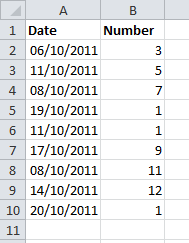
I have the following spreadsheet which I'll refer to as Spreadsheet A
and this spreadsheet which I will refer to as Spreadsheet B
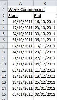
I would like to write a formula which sits on each row on Spreadsheet B (i.e. row 3 downwards) and using the dates in column A and B on the same row as the formula sits looks at Column A of spreadsheet A and matches all dates that fall between the two. I would like then for all the dates that are matched on Spreadsheet A to total up all of the hours that in column B in Spreadsheet A and just show the figure.
As an example If I had the formula in column C, row 4 it would match rows 7 and 10 on Spreadsheet A and the formula would return the total number 10 (as it adds 9 and 1).
Is this possible through SUMPRODUCT or similar?
Any help would be greatly appreciated.
GISVPN
I have the following spreadsheet which I'll refer to as Spreadsheet A
and this spreadsheet which I will refer to as Spreadsheet B
I would like to write a formula which sits on each row on Spreadsheet B (i.e. row 3 downwards) and using the dates in column A and B on the same row as the formula sits looks at Column A of spreadsheet A and matches all dates that fall between the two. I would like then for all the dates that are matched on Spreadsheet A to total up all of the hours that in column B in Spreadsheet A and just show the figure.
As an example If I had the formula in column C, row 4 it would match rows 7 and 10 on Spreadsheet A and the formula would return the total number 10 (as it adds 9 and 1).
Is this possible through SUMPRODUCT or similar?
Any help would be greatly appreciated.
GISVPN
SOLUTION
membership
This solution is only available to members.
To access this solution, you must be a member of Experts Exchange.
ASKER CERTIFIED SOLUTION
membership
This solution is only available to members.
To access this solution, you must be a member of Experts Exchange.
SOLUTION
membership
This solution is only available to members.
To access this solution, you must be a member of Experts Exchange.
ASKER
Could you explain why the second SUMIF (SUMIF(Sheet1!A:A,">"&B1,S
Regards,
GISVPN