asked on

Excel - Vlookup Array with date

Hello expets,

I need help with an Array. Not sure what the issue is, but I can't do an array if the data in the column is date or number only.

I have first sheet that pulls data from database. Worksheet 2 is "Comment". It looks at column A and B to do a lookup and then display data from column F if it match. It works if I put text and numbers. However, it will not work if my column F are dates. Is there something wrong with the lookup that it's causing it to not work with date?

=LOOKUP("ZZZ", IF({1,0}, "", INDEX(COMMENT!F$1:F$9936, MATCH(1,(A2=COMMENT!A$1:A$9936)*(B2=COMMENT!B$1:B$9936),0))))

Jacques Geday

can you post sample where you have the data ?
gowflow

ASKER CERTIFIED SOLUTION

barry houdini

membership

This solution is only available to members.

To access this solution, you must be a member of Experts Exchange.

Start Free Trial

holemania

ASKER

Not sure if this will help, but attached are 2 screenshot. I have the "master" worksheet that is data is pulled from database. No one is to do anything with this one since data can change when refresh. Then I have "comment" worksheet that allow the user to type in comments. Worksheet "Master" has the lookup to "comment" and pull that into "Master". The Scrap and Comments column work. However, my Date column isn't carrying over.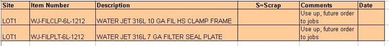

COMMENT.jpg

holemania

ASKER

barryhoudini,

That seems to work. The 2nd one actually works well.

Is it possible to modify it so that I don't have to specify the cells to find?

Example:
=IF(SUM((A=COMMENT!A:A)*(B=COMMENT!B:B)),INDEX(COMMENT!F:F, MATCH(1,(A=COMMENT!A:A)*(B=COMMENT!B:B),0)),"")

So look at the master list for all in column A and match with comment list. Then do it for B from master list to comment list and display column F?

Hoping not have to hard code which cell to search and range. Would that work? I tried it but it's showing nothing.

barry houdini

No, In Excel 2003 you'll need to keep specific ranges, rather than whole columns......

regards, barry

holemania

ASKER

Thanks. Using your example:

=IF(SUM((A2=COMMENT!A$1:A$9936)*(B2=COMMENT!B$1:B$9936)),INDEX(COMMENT!F$1:F$9936, MATCH(1,(A2=COMMENT!A$1:A$9936)*(B2=COMMENT!B$1:B$9936),0)),"")

If my Master worksheet has nothing in Column A and B, the date is showing as 1/0/1900. Is there any way to set it so that it's not doing that and make it blank instead?

barry houdini

As per my comment in first answer, custom format like this

custom format result cell as m/d/yyyy;;

Note the two semi-colons at the end, if you include those then zeroes are shown as blanks

regards, barry

holemania

ASKER

Awesome. Thank you so much for your help. Awarding you points.

Hopefully you can help answer a quick question in regard to the same lookup. I'm doing a reverse lookup from "Comment" worksheet back to "Master" worksheet. I am checking and see if Column A and B from "Comment" worksheet match "Master" worksheet. If not, put in X in column G in "Comment" worksheet to indicate that the item doesn't exist.

Taking your example, again, would hard coding "X" it in there work? It's showing up blank.

=IF(SUM((A2=MASTER!A$1:A$9936)*(B2=MASTER!B$1:B$9936)),INDEX("X", MATCH(1,(A2=MASTER!A$1:A$9936)*(B2=MASTER!B$1:B$9936),0)),"")

barry houdini

Is that last formula simply required to see if there's a match?....or do you want to retrieve a specific value? What should the formula return if there is a matching row?

regards, barry

holemania

ASKER

If it matches, to return blank. However, if it doesn't match to mark it with an "X" in the Comment worksheet so user know that the item doesn't exists any more.

I can return data, but I just want to have it return an "X". I tried putting "X" in there, but it's not doing anything. It's pulling blank.

barry houdini

Try like this

=IF(SUMPRODUCT((A2=MASTER!A$1:A$9936)*(B2=MASTER!B$1:B$9936)),"","X")

regards, barry

holemania

ASKER

Thank you. That worked great.