Referencing Pivot Table Ranges in VBA in Excel 2010 for Conditional Formatting
Hello,
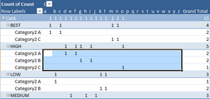
I would like to know how select a range of cells (using VBA) within a Pivot Table that belong to a specific category please. (as seen in the screenshot below)
 My aim is to programmatically give those cells with a "1" a different colour based on the level of importance. For example HIGH will be red, and MEDIUM will be orange. This pic shows how I want the end result to look like:
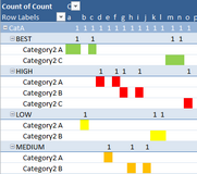 The reason why this needs to be done in VBA is because I create many pivot tables based on the same categories but with different data. There could be many more rows within HIGH or a different number of columns based on the data source, so it needs a PivotTable VBA command that knows the chart's boundaries so that the relevant conditional formatting can be applied.
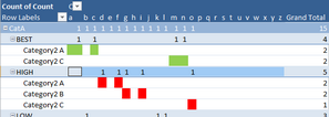
What I have figured out so far is the ability to select cells based on their category using the VBA code below, but the issue is it selects category totals rather than all cells within a category (screenshot below shows what the code actually selects, which are the cells to the right of HIGH)
 I'm hoping someone on here has the technical know-how to help solve this please?
Attached is a temporary .xlsm which has my raw data (test values for this purpose), the pivot table, and the VBA code which does the selection.
PivotSelect.xlsm
Many thanks in advance,
Paul.
I would like to know how select a range of cells (using VBA) within a Pivot Table that belong to a specific category please. (as seen in the screenshot below)
My aim is to programmatically give those cells with a "1" a different colour based on the level of importance. For example HIGH will be red, and MEDIUM will be orange. This pic shows how I want the end result to look like:The reason why this needs to be done in VBA is because I create many pivot tables based on the same categories but with different data. There could be many more rows within HIGH or a different number of columns based on the data source, so it needs a PivotTable VBA command that knows the chart's boundaries so that the relevant conditional formatting can be applied.What I have figured out so far is the ability to select cells based on their category using the VBA code below, but the issue is it selects category totals rather than all cells within a category (screenshot below shows what the code actually selects, which are the cells to the right of HIGH)
Dim pt As PivotTable
Set pt = ActiveSheet.PivotTables(1)
pt.PivotFields("Level").PivotItems("HIGH").DataRange.SelectAttached is a temporary .xlsm which has my raw data (test values for this purpose), the pivot table, and the VBA code which does the selection.
PivotSelect.xlsm
Many thanks in advance,
Paul.
ASKER CERTIFIED SOLUTION
membership
This solution is only available to members.
To access this solution, you must be a member of Experts Exchange.
ASKER
Got it:
pvtItem.DataRange.SpecialC
Thanks very much for your help!!!
pvtItem.DataRange.SpecialC
Thanks very much for your help!!!
Hi
Glad you sorted out yourself. :)
Kris
Glad you sorted out yourself. :)
Kris
ASKER
Hi Kris,
I have one more question for a very similar issue using the same Pivot table that I'm hoping you may be able to help with please?
http://www.experts-exchang
I have one more question for a very similar issue using the same Pivot table that I'm hoping you may be able to help with please?
http://www.experts-exchang
ASKER
Thank you very much, your code does exactly what I was after! I see what you've done in that for it to detect the correct BEST/HIGH, etc field you had to change the layout to Tabular so that the correct cells could be highlighted and modified. Great idea, never thought of that!!
To turn the layout back to compact view I know I can just add the following code:
ActiveSheet.PivotTables("P
However, one quick question please before I mark it as a definate answer, what is the code to change the font colour as well please? I would like the cell to be purely the colour needed so the value "1" needs to match the background colour as well please.
Thanks,
Paul.