dungla2012
asked on
How to do this!
How to do this work
Thank you!
Thank you!
That was not a very useful title for a question. These titles help the experts to pick questions which they can address best. Also to access the asked questions the titles are the main identification to what could be the content in the question and also help people find questions close to their needs.
ASKER CERTIFIED SOLUTION
membership
This solution is only available to members.
To access this solution, you must be a member of Experts Exchange.
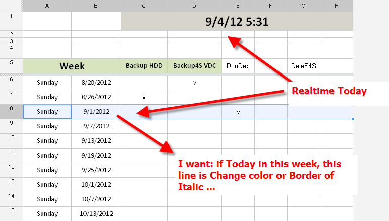
Select the who;e rows from 6 onwards and add a new conditional formatting rule with the formula
=IF(AND($C$1-$B6<7,$C$1-$B6>=0),TRUE,FALSE)
Slight tweak to andrewssd3's suggestion, you can use the FLOOR function:
=FLOOR($C$1,7)=$B6
The conditional formatting is looking for a TRUE or FALSE result, the formula above will give a TRUE or FALSE without needing the IF statement above.
The FLOOR function rounds a number down to the specified factor, in this instance rounding down to the previous mulitple of 7. This is because Excel stores dates as a serial number of number of days since 01/01/1900 with Saturday being the day 7 of each group (week), therefore multiples of 7 will be consecutive Saturdays.
Your sheet above shows a little inconsistency, the day shows Sunday but 9/1/2012 (assuming 1st September) was a Saturday.
Thanks
Rob H
http://www.cpearson.com/excel/cformatting.htm