CG4444
asked on
How conditionally format elements of a Pivot Table base their value
Hi there!, I need help with a macro to conditional format a Pivot Table (Pivot1) cells base in their values;
The table (pic1) have columns; Item, SubItem, Item_Child, Code and Qty.
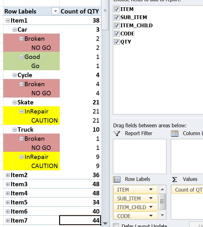
The Pivot(pic2) is a count of Items, the Items can be a Car, Truck, Bike, or Skate. These Items can be “Broken”= NO GO “Good”= GO or “InRepair”= CAUTION.
What I want is to dynamically probably on the Sheet Change event conditionally format(pic3) if it’s NO GO background color = Red, if its Go green and CAUTION yellow. I need the cells of the Items be these color but not just where the words “GO-NO GO-CAUTION” but the “condition” of Item(GO-NO_GO-CAUTION) and the “Stage” of the Item(Broken-Good-InRepair)
Can someone please help me with this code?
I really appreciate this help.
Thanks.
The table (pic1) have columns; Item, SubItem, Item_Child, Code and Qty.
The Pivot(pic2) is a count of Items, the Items can be a Car, Truck, Bike, or Skate. These Items can be “Broken”= NO GO “Good”= GO or “InRepair”= CAUTION.
What I want is to dynamically probably on the Sheet Change event conditionally format(pic3) if it’s NO GO background color = Red, if its Go green and CAUTION yellow. I need the cells of the Items be these color but not just where the words “GO-NO GO-CAUTION” but the “condition” of Item(GO-NO_GO-CAUTION) and the “Stage” of the Item(Broken-Good-InRepair)
Can someone please help me with this code?
I really appreciate this help.
Thanks.
ASKER
Excel 2007..let me see why the pic didnt attached..
ASKER
Pivot Pic
Pivot1.bmp
Pivot1.bmp
Option Explicit

Sub FormatPivotTable()
    Dim c As Range
    With ActiveSheet.PivotTables("pic3")

        ' reset default formatting
        With .TableRange1
            .Interior.ColorIndex = 0
        End With

        ' apply formatting to each row if condition is met
        For Each c In .DataBodyRange.Cells
            Select Case c.Value
                Case Is = "NO GO"
                    With .TableRange1.Rows(c.Row - .TableRange1.Row + 1)
                        .Interior.ColorIndex = 3
                    End With
                Case Is = "GO"
                    With .TableRange1.Rows(c.Row - .TableRange1.Row + 1)
                        .Interior.ColorIndex = 4
                    End With
                Case Is = "CAUTION"
                    With .TableRange1.Rows(c.Row - .TableRange1.Row + 1)
                        .Interior.ColorIndex = 6
                    End With
            End Select
        Next

    End With
End Sub

Private Sub Worksheet_PivotTableUpdate(ByVal Target As PivotTable)
    If Target.Name = "pic3" Then
        FormatPivotTable
    End If
End SubASKER
jkasavan
MacroShadow
I appreciate your help.
I tried the code and something strange happened, it did flashed the color and then It just doesn’t apply the colors. I’m attaching the workbook.
Pivot1.xlsm
MacroShadow
I appreciate your help.
I tried the code and something strange happened, it did flashed the color and then It just doesn’t apply the colors. I’m attaching the workbook.
Pivot1.xlsm
In Excel 2010, the following tweak to MacroShadow's code is working for me when you refresh the PivotTable. I changed the For...Next loop to use .RowRange.Cells
Sub FormatPivotTable()
    Dim c As Range
    Application.ScreenUpdating = False
    With ActiveSheet.PivotTables("PivotTable1")
        ' reset default formatting
        With .TableRange1
            .Interior.ColorIndex = 0
        End With

        ' apply formatting to each row if condition is met
        For Each c In .RowRange.Cells
            Select Case c.Value
                Case Is = "NOGO"
                    With .TableRange1.Rows(c.Row - .TableRange1.Row + 1)
                        .Interior.ColorIndex = 3
                    End With
                Case Is = "GO"
                    With .TableRange1.Rows(c.Row - .TableRange1.Row + 1)
                        .Interior.ColorIndex = 4
                    End With
                Case Is = "CAUTION"
                    With .TableRange1.Rows(c.Row - .TableRange1.Row + 1)
                        .Interior.ColorIndex = 6
                    End With
            End Select
        Next

    End With
End SubASKER
First of all, I apologize for uploading a 2010 workbook (uploaded from my home machine my intention is to use it in a work machine from work with ’07).
Why will it the code behave different in a 2010 Excel workbook from using the same VBA code in ‘07?
Ok. About the code, my intention is to conditionally format the cell with the words (Go-NO GO-CAUTION) but I also need what is related to these words (InRepair-Broken-Good) that initially was my main problem because I can accomplish the formatting of the words(Go-NO Go-CAUTION) without VBA. How can I reference these in the code to color the same color as (Go-NO GO-CAUTION)?
Thanks again fro the help...
If you would like to do this without using VBA:
Apply conditional formatting rule to the ENTIRE column.
1. Select the ENTIRE column.
2. Select Conditional Formatting from the Home tab.
3. Select "Format only cells that contain"
4. In the "Edit the Rule Description", change the drop down under "Format only cells with:" from CELL VALUE to SPECIFIC TEXT.
5. Make sure the comparison says "containing"
6. In the right side of the comparison type in ="Broken" (include the "=" sign).
7. Click the format button, and on the fill tab select the red fill color.
8. Click OK, then click OK.
Then create additional rules to apply the format for the green and yellow background colors.
Here is the file with these rules.
Pivot2.xlsm
Pivot2.xlsm
ASKER
One more question how can I replace .ColorIndex in the TableRange1.Rows. Interior.ColorIndex to tone down the Index bright colors for a RGB color?
ASKER
< If you would like to do this without using VBA:>
No, I do want to use VBA..
My issues cannot be accomplish without VBA.
If you look at my original post I need the 2 properties of the “Item” conditionally formatted colored, your initial code only does 1 the words sets (GO-NO GO-CAUTION) I also the need the corresponding (Good-Broken-In Repair) Please take a look at my original request.
ASKER
 This is what I need;
ASKER
jkasavan
Don’t forget that I will be using Excel 2007 at work and only 3 Cond. Format are allowed. thats the reason I need to do it in VBA. The pic posted explain better what I need to acomplish.
MacroShadow
Thanks for the link.
Don’t forget that I will be using Excel 2007 at work and only 3 Cond. Format are allowed. thats the reason I need to do it in VBA. The pic posted explain better what I need to acomplish.
MacroShadow
Thanks for the link.
Option Explicit

Sub FormatPivotTable()
    Dim c As Range
    Application.ScreenUpdating = False
    With ActiveSheet.PivotTables("PivotTable1")
        ' reset default formatting
        With .TableRange1
            .Interior.ColorIndex = 0
        End With

        ' apply formatting to each row if condition is met
        For Each c In .RowRange.Cells
            Select Case c.Value
                Case Is = "NO GO", "Broken"
                    With .TableRange1.Rows(c.Row - .TableRange1.Row + 1)
                        .Interior.ColorIndex = 3
                    End With
                Case Is = "Go", "Good"
                    With .TableRange1.Rows(c.Row - .TableRange1.Row + 1)
                        .Interior.ColorIndex = 4
                    End With
                Case Is = "CAUTION", "InRepair"
                    With .TableRange1.Rows(c.Row - .TableRange1.Row + 1)
                        .Interior.ColorIndex = 6
                    End With
            End Select
        Next

    End With
End Sub

Private Sub Worksheet_PivotTableUpdate(ByVal Target As PivotTable)
    If Target.Name = "PivotTable1" Then
        FormatPivotTable
    End If
End SubASKER
jkasavan
MacroShadow
Last suggestion;
How with the code you provided how I can reference the cell above in the code below to be color the same color. I don’t want to get more in details but in the real project the words (GO-NO GO-CAUTION) are constant static but not the (Good-Broken-InRepair) so I can not go like this ;
Case Is = "GO",Good. Etc. etc. etc. etc. ……
……so with the code you provided ( I really appreciate your help) how can I modify it so If the cell in row equals GO colored Green, BUT also the one above color it green too( no matter what the text on it is). Just help me modify this and I’ll do the rest.
Case Is = "GO"
With .TableRange1.Rows(c.Row - .TableRange1.Row + 1)
.Interior.ColorIndex = 4
End With
ASKER CERTIFIED SOLUTION
membership
This solution is only available to members.
To access this solution, you must be a member of Experts Exchange.
ASKER
Thanks a lot for your help and been patient with my explanation of request.
Glad to be of assistance.
Hi, CG4444
Actually Excel 2007 allows you to specify as many conditional formats as you like.
Actually Excel 2007 allows you to specify as many conditional formats as you like.
Which version of Excel is this? Also - the images aren't attached?