gigifarrow
asked on
Need help writing a formula that shows red when date is 30 days closer to today's date.
I have a code that looks like this: =B2<TODAY() .I need it to turn red when it is close to 30 days close to todays date.
I tried this: =B2=30Today() which of course doesnt work.
I tried this: =B2=30Today() which of course doesnt work.
If you are worrying about a shipping date, then you might want a Conditional Formatting formula like:
=B2-TODAY()<=30 'Highlight when project is 30 days or less from being due
If you are worrying about overdue invoices, then you might want a Conditional Formatting formula like:
=TODAY()-B2>=30 'Highlight when invoice is 30 days or more overdue
=B2-TODAY()<=30 'Highlight when project is 30 days or less from being due
If you are worrying about overdue invoices, then you might want a Conditional Formatting formula like:
=TODAY()-B2>=30 'Highlight when invoice is 30 days or more overdue
ASKER
Thank u is this for one field or a whole columm? If not how would you do it for more than one field
If you want multiple cells on the same row to be highlighted, then you need to put a $ in front of the B:
=$B2-TODAY()<=30 'Highlight when project is 30 days or less from being due
=TODAY()-$B2>=30 'Highlight when invoice is 30 days or more overdue
Similarly, if you want multiple cells in the same column to be highlighted, then you need to put a $ in front of the row number 2.
=$B2-TODAY()<=30 'Highlight when project is 30 days or less from being due
=TODAY()-$B2>=30 'Highlight when invoice is 30 days or more overdue
Similarly, if you want multiple cells in the same column to be highlighted, then you need to put a $ in front of the row number 2.
ASKER
I tried both of these code and get a circular refrence warnig. It also does not turn the field red.
=$B2-TODAY()<=30 'Highlight when project is 30 days or less from being due
=TODAY()-$B2>=30 'Highlight when invoice is 30 days or more overdue
=$B2-TODAY()<=30 'Highlight when project is 30 days or less from being due
=TODAY()-$B2>=30 'Highlight when invoice is 30 days or more overdue
gigifarrow,
The circular reference warning occurred because you put the formulas in the wrong place. They are intended for use in Conditional Formatting, which you will find on the Home menu in the ribbon.
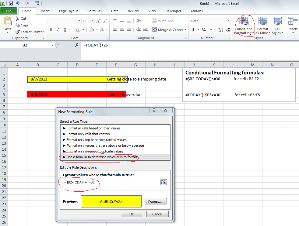
In the screenshot below, I applied a yellow conditional formatting highlight to cells B2:F2 using the first formula, and a red one to cells B5:F5 using the second.

To apply conditional formatting:
1. Select the cells that will receive the formatting
2. Open the Home...Conditional Formatting menu item
3. Click the button in the resulting dialog for "New Rule..."
4. Choose "Use a formula to determine which cells to format" in the next dialog
5. Enter the formula, then click the Format... button
6. Go to the Interior tab, then click your desired highlight color
7. Click OK twice
The circular reference warning occurred because you put the formulas in the wrong place. They are intended for use in Conditional Formatting, which you will find on the Home menu in the ribbon.
In the screenshot below, I applied a yellow conditional formatting highlight to cells B2:F2 using the first formula, and a red one to cells B5:F5 using the second.
To apply conditional formatting:
1. Select the cells that will receive the formatting
2. Open the Home...Conditional Formatting menu item
3. Click the button in the resulting dialog for "New Rule..."
4. Choose "Use a formula to determine which cells to format" in the next dialog
5. Enter the formula, then click the Format... button
6. Go to the Interior tab, then click your desired highlight color
7. Click OK twice
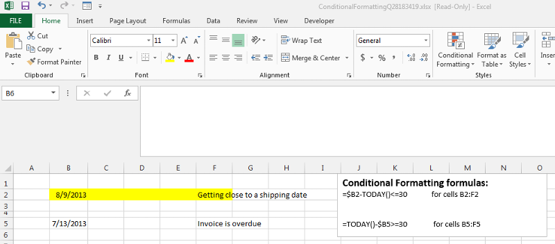
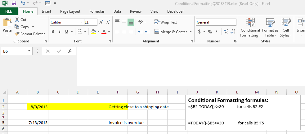
Here's a sample workbook with the Conditional Formatting in place:
ConditionalFormattingQ28183419.xlsx
ConditionalFormattingQ28183419.xlsx
ASKER
first thanks for your time.
I did exactly what you said and once I hit Ok twice, the format I selected which is yellow turns all the selected fields to the formatted color of yellow.
It changes to white when I put 7/15/2013 dates in I used this one =TODAY()-$P1>=30
I only want the fields to be yellow if the date is over thirty days. I dont want it to automatically change yellow and turn white when it is less than 30 days expired.
When I go to your example and put a date in C5 it stays red. I put 07/13/13 which is not greater than equal to thirty days expired. So it shouldnt be red. It looks like yours is not working.
The conditional formatting is checking the value in cell B5. Was the reference to cell C5 a typo?
 ConditionalFormattingQ28183419.xlsx
 ConditionalFormattingQ28183419.xlsx
ASKER
I thought you selected B5 thru F5 so it should work on C5 because that is what you have in your note that was selected.
"Why is the whole line yellow when you havent put a date in the other fields?
It only works for that one field B2 none of the other in B2 thru F2.
"Why is the whole line yellow when you havent put a date in the other fields?
It only works for that one field B2 none of the other in B2 thru F2.
ASKER CERTIFIED SOLUTION
membership
This solution is only available to members.
To access this solution, you must be a member of Experts Exchange.
Sorry, I think I am misunderstanding your exact requirements.
Do you need cell [B2] to be shown in a red forecolo(u)r when today's date is within 30 days of the date within that cell?
Please can you clarify?
Thank you.
BFN,
fp.