asked on

Excel vba to apply formats to cells in a pivot table based on a value

Hi,

I have a pivot table that consists of a number of columns and 1 row label
The row label is a date.

Basically I want to change the color of the row base on the value in the row label.
The number of rows can change on refresh. The columns are constant
The 1st row is always 'Late last month'
The last row is always 'Future Next Month'

i.e

Row Column (B) Column (D)

3 07/11/2013 (cell B3 outside pivot table)

provottable1
Due Date Val1
8 Late Last Month 1
9 27/10/2013 1
10 28/10/2013 2
11 29/10/2013 4
12 30/10/2013 0
13 31/10/2013 8
14 01/11/2013 0
15 02/11/2013 1
16 03/11/2013 4
17 04/11/2013 4
18 05/11/2013 0
19 06/11/2013 9
20 07/11/2013 0
21 08/11/2013 6
21 09/11/2013 4
24 10/11/2013 5
25 11/11/2013 4
26 12/11/2013 8
27 13/11/2013 5
28 14/11/2013 5
29 15/11/2013 6
30 16/11/2013 4
31 17/11/2013 5
32 18/11/2013 3
33 19/11/2013 4
34 20/11/2013 8
35 21/11/2013 7
36 22/11/2013 2
37 23/11/2013 4
38 Future Next Month 12

I see the steps as being as follows but I'm not particularly good at VBA

1. Enter the Table and clear any existing formats.

2. find the last row that needs to to formatted in the pivottable.
Go to the row that contains 'Future Next Month' in column B of the table
Loop back until the Due Date is < the date set outside the pivot in cell B3
(that would equate to row 19)

3 Highlight from last row found to row 19 back to row 9 . (columns B and D)

4. Change the color

I've seen various forums about this but none do what I want and all the examples use different methods that I can't combine.

hope you can help

terencino

Have you considered conditional formatting for this task? If you like to send a sample table and the colours you want for the cells than I can show you how it would apply in this situation
...Terry

Hamed Nasr

Try to reproduce the issue and upload the sheet.
Give example of how you expect the output.
Example look as cell x, y. The label is label1, I expect the color to be ....

Faustulus

Any solution to your problem will have to be custom made. It will work only on your workbook. Therefore it can't be made without access to your workbook. You can replace proprietary data with dummies of identical data type.

Eric Harris

ASKER

Yes I've tried condition formatting but it too erratic.
I'm looking for a vba solution

It's a biggy so impossible to post.
I was hoping there was enough information there to have a stab so that I can adopt it to fit.

Aah well, worth a try.

Faustulus

Post the first 20 rows.

Eric Harris

ASKER

Here's an extract of the file.

The pivot is refreshed by users each day a macro to sql connections

I want to change the color of columns B, D,E,F,F to be red only affecting rows where the due date less than the date in cell C2
The values are made up so it's ok to mess around

Cheers
Daily-Order-and-Sales.xlsm

terencino

Those cells are formatted as text not dates, which is why conditional formatting hasn't worked before. Here is an update using conditional formatting attached, using DATEVALUE to convert text to date
...Terry
Daily-Order-and-Sales.xlsm

Eric Harris

ASKER

I did try Conditional formatting but I encountered problems when I did the data refresh and the subsequent pivot refresh.
Each time I refresh the pivot the formatting is lost.

ASKER CERTIFIED SOLUTION

terencino

membership

This solution is only available to members.

To access this solution, you must be a member of Experts Exchange.

Start Free Trial

Eric Harris

ASKER

Thatg is truly Amazing
You my friend are a wizard
It works a treat.

I an see what you have done but wondered how you got the formats to hold after the refresh.

Thanks

terencino

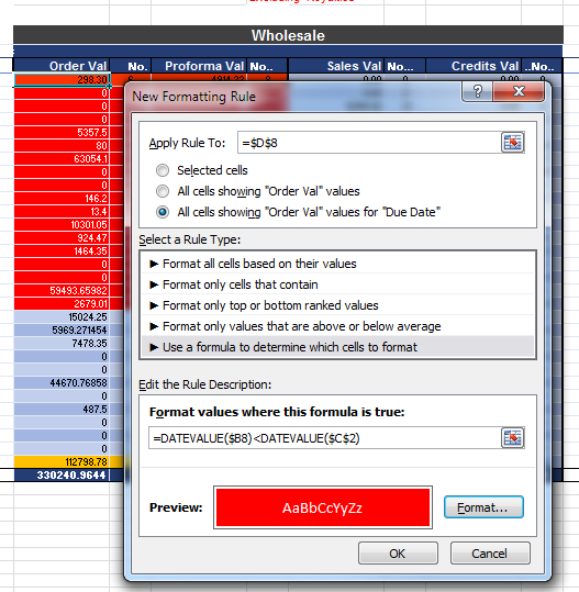
Great the trick is to apply the conditional formats to individual columns in the values section of the pivot table. So :
1. Select D8, the first value in the first column of the Values section of the pivot table
2. Click on Conditional Formatting > New Rule and select "All cells showing Order Val values for Due Date". This will ignore subtotals and grand totals. Also, it will expand automatically on refresh, as the conditional formatting is locked to the pivot table, not the cells below.
3. Select the Rule Type "Use a formula..." and enter the formula
=DATEVALUE($B8)<DATEVALUE($C$2)
This will be TRUE for the required dates, and FALSE or an error for other entries, which will be ignored. The referencing is less important for these pivot table formats, but essential for the normal range formats, so I have kept it the same throughout.
4. Change the format to suit
5. Repeat for all the other Values columns
6. For the Row Label Due Date, it should be treated the same as a normal range. Just select all the cells starting from B8 to B51 that are likely to be included in a refresh, and select a formula and add the conditional formula above.

terencino

Also, here is the chapter & verse from Microsoft on using conditional formatting with pivot tables:

Add, change, find, or clear conditional formats

Eric Harris

ASKER

Excellent.
I have tweaked based on what you have done and added formats to other columns.

Thanks you so much for your help.
It is much appreciated.