Math in Macro needs fix
EE Pros,
I have a Risk/Return Macro and chart that when you put two variables into each cell in a row, it plots the appropriate point on the grid. Here's the issue. When you prioritize the list, (it sorts the descriptions, it doesn't properly calculate the sort. In other words a Return of 8 and a Risk factor of 4 should take priority over a Return of 9 and a Risk factor of 6.
Look at the WS to see what I'm trying to accomplish.
Thank you in advance.
B.
Math-in-Macro-is-incorrect.xlsm
Martin Liss
When I click the button nothing happens perhaps because I'm missing some links. What happens when you click the button and what should happen if it were working correctly.
ASKER
Marty,
Thanks for taking a look...... Change the values in col. C and D and then hit prioritize. It will then stack rank the text in the order of priority. The problem I have is that it seems to prioritize the first value but it doesn't seem to properly rank the other values. A 5 on Return with a 5 on Risk should be higher up then a 5 on Return with a 6 on Risk.
Make sense?
B.
That formula is too complex for me to analyze but if you can describe the formula's logic in words, perhaps I can come up with a VBA solution.
ASKER
Much thanks.
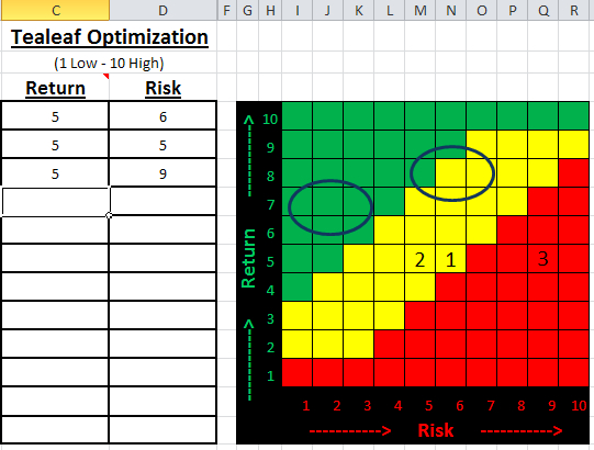
So, I think the best way to look at this is that there are two axis's that scale in opposite directions. What happens is that a description is put into Column B. Then a Return value and a Risk value are placed into Columns C (Return) and Column D (Risk). The higher the number (1-10) in the Return axis, the more value. The lower the number (1-10) in the Risk axis (D), the more value. So the most valuable combination would be 10 (C) and 1(D) while the lowest value would be a 1(C) and a 10(D). With that as potentially an array, every combined value should be able to be prioritized (and reordered in Column B.
You will see that the model actually works well.....EXCEPT for the fact that the math doesn't completely work. In the example I sent you, the order should be B, C and A when the Prioritize macro is fired.
Make sense?
B.
If this isn't correct please tell me where the 1, 2 and 3 should go.
Your "ranking" formula in column E is favoring higher risk rather than lower risk because you are adding the value in D7:
=(C7*2)+D7
If you subtract the value in D7, then the formula will favor lower risk over higher risk:
=(C7*2)-D7
=(C7*2)+D7
If you subtract the value in D7, then the formula will favor lower risk over higher risk:
=(C7*2)-D7
ASKER
Marty,
1 and 2 should be switched as they are prioritized. 1 has more value because while the return is =, the risk is lower. When that is determined, the graphic should show "1" as the best option and also have sorted the description and values in the table.
Make sense?
B.
1 and 2 should be switched as they are prioritized. 1 has more value because while the return is =, the risk is lower. When that is determined, the graphic should show "1" as the best option and also have sorted the description and values in the table.
Make sense?
B.
SOLUTION
membership
This solution is only available to members.
To access this solution, you must be a member of Experts Exchange.
ASKER CERTIFIED SOLUTION
membership
This solution is only available to members.
To access this solution, you must be a member of Experts Exchange.
ASKER
Brad and Marty,
Thanks guys! Based on the input you gave me, I was able to figure it out on my own!
Here's what I ended up doing. It was a long time ago that this graphic was made so I had missed the fact that I had a row hidden. By unhiding the "helper" row, I changed the formula to =if(b="",0,(c + (10-d))) and it works perfectly when "priority" is fired.
Thanks again,
B.
The original formula in column E weighted the Return twice as much as the Risk. Your revised formula assigns equal weighting to Return and Risk. Was this change in philosophy intentional?
From a ranking point of view, it doesn't matter whether you add the 10 or not. Even though the following two formulas return different results, they will make your rows sort exactly the same:
=IF(b="",0,c + (10-d))
=IF(b="",0,c-d)
The value returned by the first formula (on rows with data) will always be exactly 10 higher than the value returned by the second formula. This constant difference is why either formula can be used to rank your data for a sort.
Brad
ASKER
Brad,
Great comments! I did want, in this instance, Risk and Return to be =. Graphic looks pretty good now.
Thanks again,
b.
Great comments! I did want, in this instance, Risk and Return to be =. Graphic looks pretty good now.
Thanks again,
b.