Maths2

Hi there,

Can you elaborate a bit more on your instructions? Like, a lot more? It's difficult at best to follow what you want.

There is different formulas for High & low

What does this mean? What are the different formulas? Where are they at? Does this mean anything for us?

Now find High & high date between date 2/11/2011 i.e. cell N3 (row 31)from date of very first hit which is in row 37. result will be in row 36 i.e. High 5589 2/18/2011

I think I can follow this. Still a little shaky on the details though. For example, are the dates in N3 and N4 a date range? Do you only want to find the next highest value after the date in N3? You could achieve this a couple of ways, either array-entered formula, which is confirmed with CTRL + SHIFT + ENTER, instead of just ENTER, but we'd need to know specifics. You could do this with a non-array entered formula as well, but again, more specifics are needed.

We need clear and concise explanations to give you any sort of help. Please list them out in a post and not in an attached file. In a file attachment we'd really only like to see two things, 1) the data as you have it to start, and 2) the desired outcome. All directions and instructions should be in a post.

Regards,
Zack Barresse

Is this some kind of training or academic problem?

mlmcc

Hi Mr.Zack Barresse,

I know this is difficult to understand what is going on other minds i.e. my mind.as you said I had tried & mention below, what mi trying to do. please revert me back if need further clarification.

Step 1 By clicking button process start in Sheet “Data”
Step 2 if there is “High” in Cell L3 then have to find minimum value from column D from range - date in Cell N3 (which is in our case it is 1/4/2011 & it is in data table column A header ”Date” in row 4) to next Hit found.
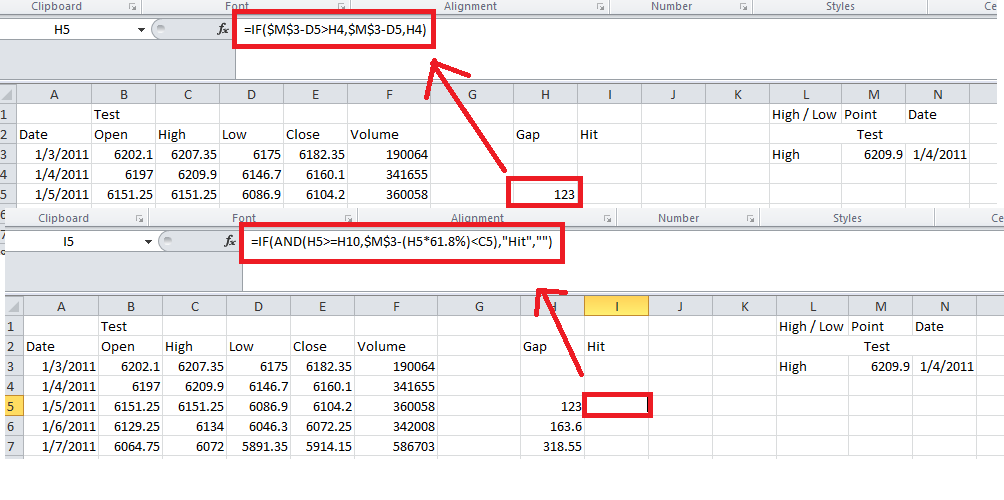
How do I get “Hit” is calculated in attached workbook –sheet – A. See Column H & I i.e. Gap & Hit. Calculation starts from one row lower from actual one.as we find Hit, have to find minimum value  From range hit row number to start date row number from column D i.e.  Header “Low”. Calculation formula for High is mentioned in cell H5 & I5 Respectively.

As we found result in cell D31 which is minimum value in that range.

Step 3 Register this result in range L3:N3 by shifting one row down all data in that column  i.e. “Low” in cell L3 5175.10 in cell M3 & 2/11/2011 in cell N3.

Step 4 now there is “Low” in cell L3 so need to find Maximum value  from this low date to next hit date. Process is the same just formula is different & have to find Max from the range i.e. column C.

Step 3
Do this till we find “Hit” but there is no data in column A i.e. end of process part one.

Arrange result in column L M N in oldest date first to latest last copy & past special value in sheet “DataBase” from row 1 to next available blank column.

in short I am finding High Value & Low value from this table form available date to Hit date where ever I found.

in attached file there is Sheet Called “High” & “Low” you can see formula difference for High & low  criteria.
Sheet “Data” is desire result I want.
Sheet “DataBase” is final result.


See attached file.

Thank You
Naresh Patel
Maths-2.xlsx

Any one on this question?

There is no way you'll get away with this as a formula.  Have you got the capability and skill to code a macro?

Nope

But it is clear now, what am I intend to do?

Naresh,

Sorry I didn't get back to you sooner, it's been busy. There is still some issues with your explanation not matching what you've said.

Before I get into this, have you ever thought of using a table? It might make this easier to work with.

Step 1 By clicking button process start in Sheet “Data”

I'm really not sure what I'm supposed to know about this step. What does this have to do with anything? Is this just a description of where you want a button to fire something off? Other than that I'm not sure what you're wanting done.

Step 2 if there is “High” in Cell L3 then have to find minimum value from column D from range - date in Cell N3 (which is in our case it is 1/4/2011 & it is in data table column A header ”Date” in row 4) to next Hit found.

Why would there be a "High' in cell L3? Do you list them there? When? How? Why? What if it isn't "High"? If I'm understanding this correctly, you will enter values in column L and N, either High or Low, and a date, and you want the corresponding high/low value returned from that date. If that is the case, the formula for that is easy and becomes...

=VLOOKUP(N3,$A:$F,LOOKUP(L3,{"Close","High","Low"},{5,3,4}),0)

Select allOpen in new window

How do I get “Hit” is calculated in attached workbook –sheet – A. See Column H & I i.e. Gap & Hit. Calculation starts from one row lower from actual one.as we find Hit, have to find minimum value  From range hit row number to start date row number from column D i.e.  Header “Low”. Calculation formula for High is mentioned in cell H5 & I5 Respectively.

This doesn't make sense.  Why not keep this as a single formula? Will the date column always be sorted in ascending order? Will this data always stay the same? On your High and Low sheets it doesn't match what you have in columns L through N on your Data sheet. Why is that?

I'm not sure if it's the language barrier, but I find almost nothing helpful about your explanation. The attached file uses a table on the Data sheet and incorporates your formulas from both sheets High and Low. Honestly I'm not sure what else you need here.

Regards,
Zack
Maths-2.xlsx

Give me some time to reply.......i am off the desk ......

Thanks

Mr.Zack,

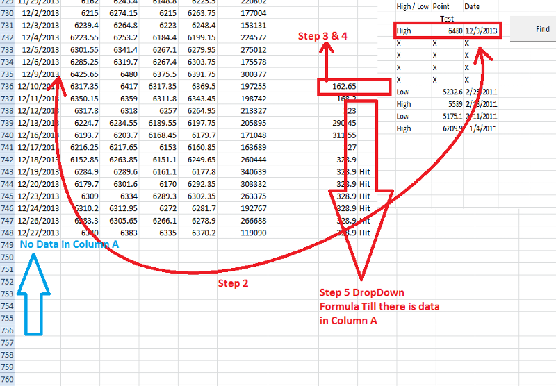
Sorry for my improper & confusing explanation. This is my last attempt to show how we achieve this. Now there is only one sheet on which we have to work on. “Data” Sheet. I had mention logic flow behind this by clicking button “Find”. One more thing there is manually typed data in rang L3:N3 for one time. So before clicking button there is data available in range L3:N3.

Logic Flow

01. Button Click

On click of button process start.

02. Find Row Number Of Date

Find row number of the date  in column A which is mention in Cell N3.

03. Putting Formula - Column H

Put formula in column H Row is Step 2 Result +1.“IF($L$3="High",IF($M$3-D5>H4,$M$3-D5,H4),IF($L$3="Low",IF(C5-$M$3>H4,C5-$M$3,H4),""))”.(assume date found in row 4) if date found in row 10 then formula will be in H column row 11(Cell H11) is “IF($L$3="High",IF($M$3-D11>H10,$M$3-D11,H10),IF($L$3="Low",IF(C11-$M$3>H10,C11-$M$3,H10),""))”.

04. Putting Formula - Column I

Put formula in column I row is Step2 row number +1. I.e. Row 5(Cell I5) assumes date found in row 4.” IF($L$3="High",IF(AND(H5>=H10,$M$3-(H5*61.8%)<C5),"Hit",""),IF($L$3="Low",IF(AND(H5>=H10,$M$3+(H5*61.8%)>D5),"Hit",""),""))” if date found in row 10 then formula will be “IF($L$3="High",IF(AND(H11>=H16,$M$3-(H11*61.8%)<C11),"Hit",""),IF($L$3="Low",IF(AND(H11>=H16,$M$3+(H11*61.8%)>D11),"Hit",""),""))” in Cell I11.

05. DropDown Of Formula

Dropdown formula till end.

06. Finding Text Hit In column I

Find Very first Hit Found in column I.

07. Part A If there is L3=High

if L3=”High” then Find lowest value from column D – Range is first row number from where we found date (Step 2) to (Step 6).

07. Part B If There is L3=Low

if L3=”Low” then Find Highest  value from column C – Range is first row number from where we found date (Step 2) to (Step 6).

08. Arrangement To Put New Result

Shift one row down data - range L3:N3.

09. Registering New Result

Copy Step 7 value & past to M3

10. Registering New Result Date

Copy past Step 7 corresponding date in N3

11. Registering High Or Low

.if L4=”High” then type “Low” in L3 & if L4=”Low” then type “High” in L3.(As we shifted one row down old data).

12. Clear Data & Formula

Clear data & formulas in column H & I

13. Next i

Step2 till Column A=””

14. End

Maths-2.xlsx
Math2.png

Regarding Tables - I know but I am not much familiar with it.


Thanks

Hi,

Thanks for the detailed steps. Did you look at the file I uploaded? If not, take a look. I'll go over the steps in more detail. I don't know if the file I uploaded will help you or not.

What I'm wondering is, the range from L3:Nx, where x is an unkown number of rows, or the last row with data (row 1 in the latest sample file, row 8 in your previous sample file), you're solving for column M, is that right? And with each new result, it should get written to columns L through N, one row per iteration? When should it stop? When no more "Hit" values are found?

Zack

Mr.Zack,
You stop at where there  is no data in column A.  Or say range A:E. So last formula drop down (step 5) till last data available in range A:E.

Thanks

Even in step 13 I had mention.


Thanks

Mr.Zack,


Any Luck..?

Mr.Zack,

You are working on this?



Thanks

I was busy today, but yes I looked at it. It's a little difficult to understand you though. You say...

You stop at where there  is no data in column A.  Or say range A:E. So last formula drop down (step 5) till last data available in range A:E.

But I'm still uncertain as to what that actually means. It doesn't make sense.

You stop at where there is no data in column A.

What do you mean? What is stopped? What data?

Or say range A:E. So last formula drop down (step 5) till last data available in range A:E.

I'm still lost with this. What formula, and what drop down? And what is the last data available in range? The last row of the table? What is the cell address you're talking about?

I'm afraid I can't really give you anymore unless I understand what you're talking about. If you can refer to specific ranges in your explanations it would help. I'm sorry, I keep trying to follow you but it's proving difficult.

Zack

Mr.Zack,

I like it 1st understand & then execute, no  problem ask your confusion as many time as you want.



Thank You

Mr. Zack,


You are still on this question?


Thanks

This needs to be done via a macro.  Have you coded anything yourself yet?  

I would start by doing it manually and record a macro as you do it.  That should give you enough code to start with and I can help you loop it once that's done

Do u want me record macro?...if yes let me try as per my understanding.....

Yes please. As per your understwnding

Sir it is out of my reach & understanding - My first preference is to do it by formula but I think it not possible via formula & I assume that  Coding is the only way out ..I don't have much knowledge in coding. So it is up to you - tell me what i have to  do to achieve this?


Thanks

i had tried twice & thrice - again & again but no result - it is like circular reference. i don't know how to deal with.

That's ok. It's late here so I'll have to look tomorrow if I can

Sure eagerly looking forward. but take my this Comment for conclusion.

ok take a look as I think i've got it but I'm not sure of the values

Press the find button to see the values copied and pushed down.

Click the reset to take you back to just one row of values
Maths-2.xlsm

Sir sure I will, i am on my way back to home.give me some time to test.

Thanks

Sir ....I guess we missed

12. Clear Data & Formula

Clear Data & Formulas in Column H & IThat is why there is to many points.


Thanks

Do you mean after its finished to just clear the gap and hit columns?

Yes Sir...& again start from step 2.     Sorry For delay in reply.


thanks

Ah please have another look as i specifically did it so you didn't need to re apply the formulas. They calculate with each iteration

I shift the old values down and write the date, value and alternate either "Low" or "High"
The formulas are all calculated before they people's repeats.

Sir Tagit,

but if we don't clear formulas then values i.e. result will defer from actual one. so after clearing have to put again formula in as per Step 2. or if you want to formulas be intact. after Step 11 - Step 2 find row number say 8 then 8-1=7, delete rows Range A3:F7 & shift data up. So after this Step 3 4  5 12 is not required .

Getting my point?

Thanks

No I don't but I'm not at my computer to test out what saying so I'll be in touch when I get there.
Maybe if you explain how you came up with the formulas it would make more sense.
From your steps above you've indicated that you just clear the formulas and put them back in after changing the date and values etc in L3:N3. If that's the case then my code should work as the formulas recalculate each time

I don't mind, if include these formula in code it self.


Before explanation  just one question - Do u know any thing about technical analysis. (Stock Market).


Thanks

if yes then I ll explain via that way or just like formulas.

No I'm sorry,  I don't but don't need to explain why you use a particular percentage but what the formula needs  to be and what it needs to include.

Ok got it but FYI 61.80% is Golden Ratio.

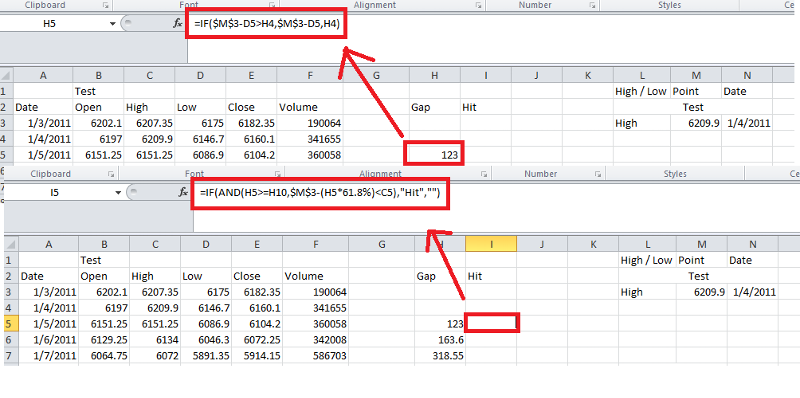
For High

IF Cell L3 = High then we are finding Lowest Low. What I did is From High i.e. M3 minus Lows of each row (Column D). & added one criteria if above value is greater than current result then above value else current value. i.e. =IF($M$3-D5>H4,$M$3-D5,H4)

& For HIT
there is 2 Criteria to match-  Criteria 1 Gap i.e. Current example Cell H5 is greater than or equal to forward 5 rows Gap i.e. Cell H10. Criteria 2 61.80% of Gap value – High point (Cell M3) is lesser High (Cell C5) then Hit else “”.
Both are matched then "Hit" else "" i.e. =IF(AND(H5>=H10,$M$3-(H5*61.8%)<C5),"Hit","").

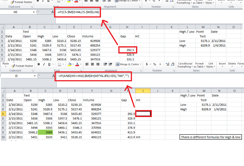
For Low

Now For Low if Cell L3=Low then finding highest high from range between low to next hit. Formula flow is like this for gap - current high (column C) - Low  (Cell M3). Here also I had add criteria previous value is greater than this value then previous value else this value. i.e. =IF(C5-$M$3>H4,C5-$M$3,H4).

For Hit two - criteria 1 forward 5 row value is greater than or equal to. Criteria 2 61.80% of Gap plus Lowest point is greater than Low (column D). i.e. =IF(AND(H5>=H10,$M$3+(H5*61.8%)>D5),"Hit","")

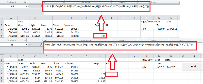
Formula Merge

And I had combine this formula if high then this if low then this else ""
For both Gap & Hit column
=IF($L$3="High",IF($M$3-D5>H4,$M$3-D5,H4),IF($L$3="Low",IF(C5-$M$3>H4,C5-$M$3,H4),""))
=IF($L$3="High",IF(AND(H5>=H10,$M$3-(H5*61.8%)<C5),"Hit",""),IF($L$3="Low",IF(AND(H5>=H10,$M$3+(H5*61.8%)>D5),"Hit",""),""))

I had attached example file in which there is sheet High & Low to see formula difference. that only for understanding only. formula merge file is math 2 in which you are working on it.

Thanks
Explanation.xlsx

Thanks for the background.  It certainly helps.

Are you saying that the formulas need to cleared and entered again from the row where the "hit" was last found?

Ok, I clear the Gap function down to the row the hit was found before continuing and it returns less values so it would be affecting the results.  the Hit formula has nothing to do with the rows above so it doesn't need to be cleared each time

Are you saying that the formulas need to cleared and entered again

Yes

from the row where the "hit" was last found?

No
 it is at =MATCH(N3,A:A,0)+1 row number in Column H & I

So in other words. Clear the formula up to and including the date in N3, found in column A

yes  :)

Ok! I'll sleep on it now as it's late.  :)

10:30 I guess ...good night...

Good morning :)

I just need to clarify about the "Hit" and the second and subsequent iterations.

Is the RANGE the rows between the Date found and the "Hit"?

And how do you know the next Date to find (Step 2)?

I think we're almost there! :)

Good Morning & Good Evening  :)
Yes Second iteration is Range the row between the date found & the Hit ...


Thanks
SO9.xlsx

Sorry wrongly attached ...pls ignore...

In Other words the new date for n3 is the corresponding row of the hit found.  Got it!
Won't be long now :)

not like that it is between lowest or highest values as per criteria between found date row & hit raw.
i.e. if we calculating from High (Cell L3 = High) for Low then we are finding Lowest value from column D range, Range =  found date row number to Hit row number & if we are calculating Low(Cell L3 =Low) then we finding Highest  value from column C - range Found date row to hit row number.

Thanks
Math2.png

Yes that makes sense.  But what is the next date we search for?  the one on the same row as hit?

no it is in the row where we found lowest or highest value from column C or D.

See the blue line in attached screen shot Step 10

& my bad I had written wrongly 2/11/2011 instead of 2/10/2011...sorry

sorry sorry    I had written right :) sorry

That's fine. Got it now. Sorry about so many questions. I just have to modify the macro slightly to work out the corresponding date of the high/low as I had it as the corresponding date for the "hit"
Brb

No Problemo, ask any number of question.....
just need to know in your new code which is you are working on it - it includes Gap & Hit column in Code it self or it is in worksheet...just asking both way I don't mind....

Thanks

The gap and hit columns are in the worksheet though I clear the formulas as I work through each iteration.  The formula itself is stored in the code.  Once we've got this working, have a look at the macro and I'll answer any questions you have

Sir rob,
Give me some time to check, as I am on way back to home,posting this comment via mobile.

Thanks

Sir rob,
What I asked for is perfectly match with your Code.row 326 - I saw there is freak trade I need to overcome with this kind of situation and rethink  different kind of formula. As manually change data and go on but it still come up with infinite in one stage where market is side ways I know may be you don't understand what I am talking.so as far as this question, this is solved.      

Thank you very much for your corporation really appreciated. I guess we will meet soon on EE again if you wish too.

Thank you and awesome.

No problem. We got there in the end. Interesting project you're working on :)

Sir rob,

I have come with change in Hit formula.. if you wish to solve it pls see my this question Math3.

Thank You