Excel Vlookup problem
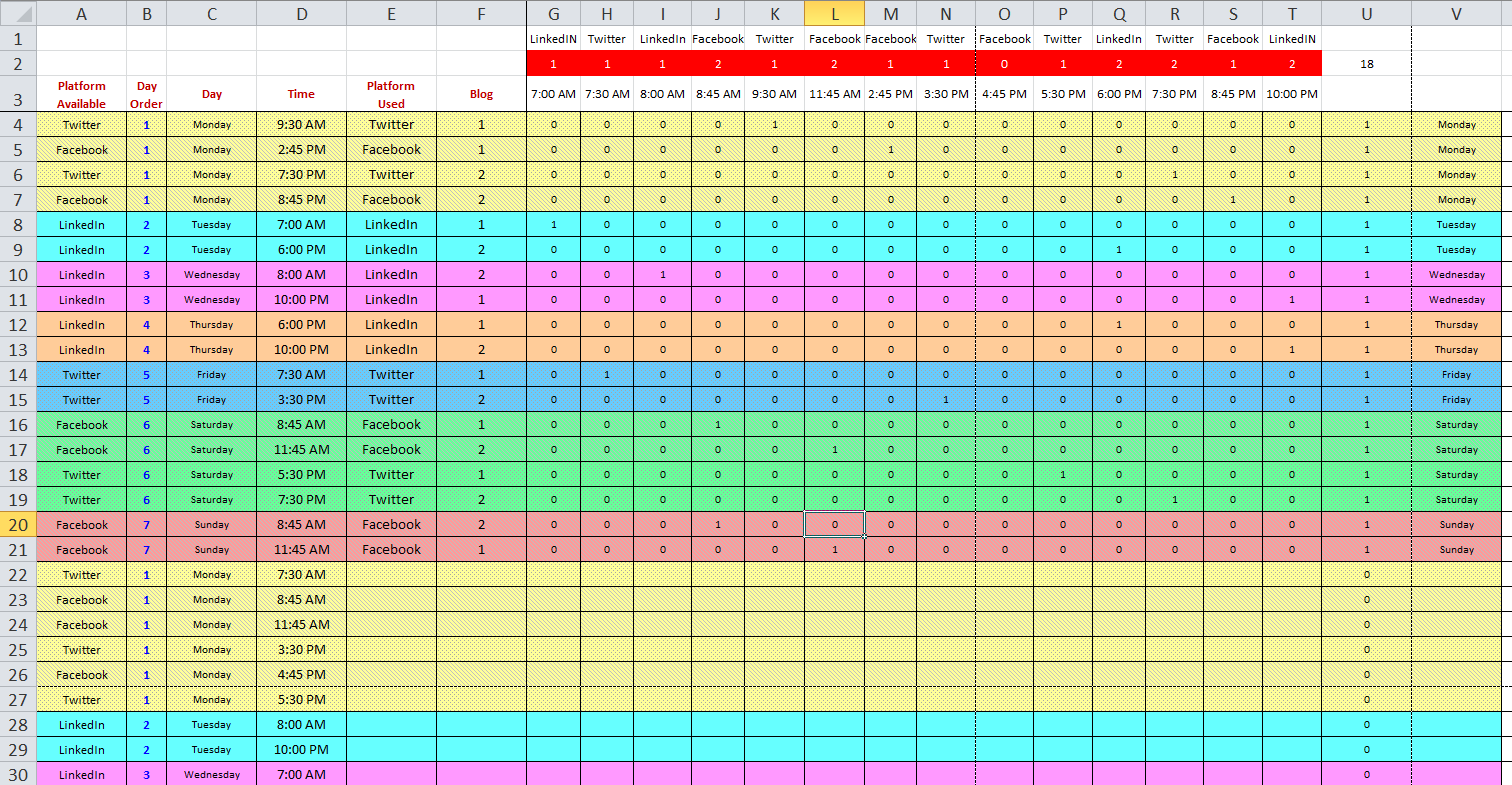
I have created a two-worksheet Excel spreadsheet. The first worksheet, Master Schedule, is a complicated looking affair where I layout my schedule of posting blogs. The columns include among others:

So one row might indicate that on Monday, at 9:30 AM, a Twitter post will be made for my first blog of that week. Across that row, in the column for 9:30 AM, a 1 will appear in that row.
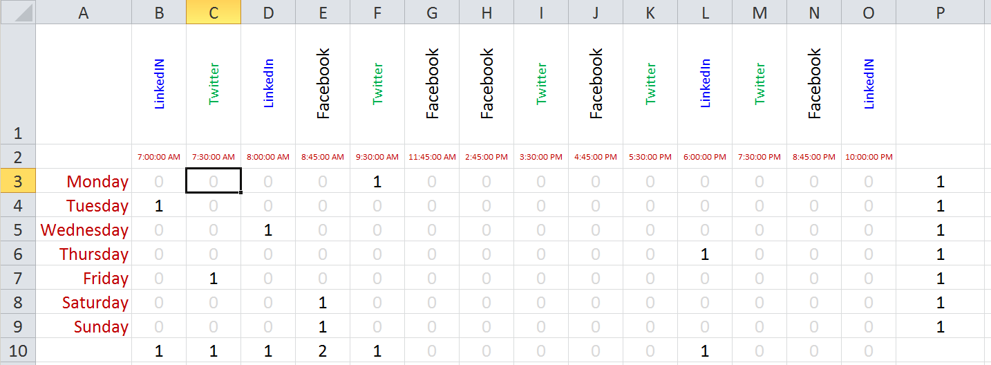
The second worksheet is where I want to create a more visual, more easily understood grid for the schedule.
The first column shows 7 rows labeled for the days of the week. Across the top are columns labeled for the platform (LinkedIn, Twitter, Facebook) and the time for the posting.
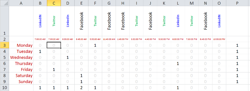
In my approach, I only post to LinkedIn at 7:00, 8:00, 18:00 and 22:00. Likewise, I only post to Twitter at 7:30, 9:30, 15:30, 17:30 and 19:30.
I'm using a Vlookup formula. Below are a few examples.
For Monday at 7:00 am, =VLOOKUP($A3,'Master Schedule'!$C$4:$T$45,5,FAL
For Monday at 7:30 am, =VLOOKUP($A3,'Master Schedule'!$C$4:$T$45,6,FAL
The problem is that my Vlookup is only working in showing the first value it finds for a posting for that day. Thus, where Monday should reflect two postings, it only shows the first one at 9:30 AM. Thursday should also show two, but it only shows the first one at 18:00. Saturday should show four, but it only shows the first one at 8:45.
What approach do I need to use to pick up all the matches? Is the answer in the function or formula or is it in how I populate the "Master Schedule" sheet.
BTW, I use the "Master Schedule" to actually create the schedule. I want the "Visual Schedule" sheet to make it easy to see what the schedule looks like.
Thanks.
Social-Networking-Schedule.xlsx
Day
Time for the posting to occur
Platform
Blog #
Plus 17 columns for the various times of day I plan on scheduling posts
Time for the posting to occur
Platform
Blog #
Plus 17 columns for the various times of day I plan on scheduling posts
So one row might indicate that on Monday, at 9:30 AM, a Twitter post will be made for my first blog of that week. Across that row, in the column for 9:30 AM, a 1 will appear in that row.
The second worksheet is where I want to create a more visual, more easily understood grid for the schedule.
The first column shows 7 rows labeled for the days of the week. Across the top are columns labeled for the platform (LinkedIn, Twitter, Facebook) and the time for the posting.
In my approach, I only post to LinkedIn at 7:00, 8:00, 18:00 and 22:00. Likewise, I only post to Twitter at 7:30, 9:30, 15:30, 17:30 and 19:30.
I'm using a Vlookup formula. Below are a few examples.
For Monday at 7:00 am, =VLOOKUP($A3,'Master Schedule'!$C$4:$T$45,5,FAL
For Monday at 7:30 am, =VLOOKUP($A3,'Master Schedule'!$C$4:$T$45,6,FAL
The problem is that my Vlookup is only working in showing the first value it finds for a posting for that day. Thus, where Monday should reflect two postings, it only shows the first one at 9:30 AM. Thursday should also show two, but it only shows the first one at 18:00. Saturday should show four, but it only shows the first one at 8:45.
What approach do I need to use to pick up all the matches? Is the answer in the function or formula or is it in how I populate the "Master Schedule" sheet.
BTW, I use the "Master Schedule" to actually create the schedule. I want the "Visual Schedule" sheet to make it easy to see what the schedule looks like.
Thanks.
Social-Networking-Schedule.xlsx
ASKER CERTIFIED SOLUTION
membership
This solution is only available to members.
To access this solution, you must be a member of Experts Exchange.
ASKER
ITJockey:
I have recreated your formula and locked in the row number so it looks like this:
=VLOOKUP($A4&TEXT(L$2,"HH:
That works in any cell where it should. Everyplace else it returns a #N/A.
What should be added to avoid that?
I have recreated your formula and locked in the row number so it looks like this:
=VLOOKUP($A4&TEXT(L$2,"HH:
That works in any cell where it should. Everyplace else it returns a #N/A.
What should be added to avoid that?
ASKER
hgholt:
Thanks for you're suggestion. My wife is calling me away right now. I'll look at that later.
Jim
Thanks for you're suggestion. My wife is calling me away right now. I'll look at that later.
Jim
ASKER
hgholt:
It works. Thanks.
It works. Thanks.
=IFERROR(as it is whole formula, "")
This will overcome with #N/A. Error is replace with "" I.e blank.
Thanks
This will overcome with #N/A. Error is replace with "" I.e blank.
Thanks
ASKER
That works. I want to accept both solutions, but give you each full points instead of splitting them. I've learned completely new things from each.
Is there a way I can do that? I'm guessing accept one here and then do something special?
Is there a way I can do that? I'm guessing accept one here and then do something special?
Mr.coachjim,
Thank You for generosity. But as per my opinion Mr.hgholt solution is more suitable then me, as in that you don't have to change anything in your Workbook. & as per standards of excel that is best way to achieve your desire result. it is my bad how do I forgot this ..... :)
Thanks
Thank You for generosity. But as per my opinion Mr.hgholt solution is more suitable then me, as in that you don't have to change anything in your Workbook. & as per standards of excel that is best way to achieve your desire result. it is my bad how do I forgot this ..... :)
Thanks
ASKER
Mr. itjockey & Mr. Hgholt
Arg! That's the sound of frustration.
I appreciate that one solution required a change to the workbook and that a solution that doesn't require a change is more elegant and sometimes critical.
But I loved both solutions and learned equally from them.
And I won't argue with you, Mr. Itjockey. You say give this one to Mr. Hgholt and I will.
I will also see if I can think of a problem to send your way.
Thanks to you both.
Jim
ASKER
This was a first for me. I've posed questions in the past where several people submitted parts of the ultimate solution and I could easily award shared solutions.
This time I got two great and totally distinct solutions. Either of which would have been great yet I end up just awarding one as the solution.
I'm delighted and bummed at the same time.
This time I got two great and totally distinct solutions. Either of which would have been great yet I end up just awarding one as the solution.
I'm delighted and bummed at the same time.
You are welcomed!!!!!
only one thing to mention ( I dint investigated yet) but if there is numerical 2 in source sheet even then COUNTIF returns with 1 or 0. And VLOOKUP returns with actual number.
I don't know how your data is in source sheet but it is just thought.
Thanks
I don't know how your data is in source sheet but it is just thought.
Thanks
ASKER
Mr. ITJockey
Good point and relevant to my application.
I'll get back to you directly on this.
Jim
Good point and relevant to my application.
I'll get back to you directly on this.
Jim
so you will get your all look up values perfect,
if you want like this then i will further help you with formula. i had enter only one cell formula in attached with yellow background.
let me know
Thanks
Social-Networking-Schedule.xlsx