Microsoft Excel
--
Questions
--
Followers
Top Experts
Finding total sales per customer, using excel
Hi,
I have a spreadsheet that has two columns
A - customer number
B - purchase amount
I would like to easily get the total amount each customer paid. It would also be nice to see this data in descending order, from the customer who paid the most to the least, if possible.
How can this be done? Please provide an example.
Please see the attached file. (all bogus data, but basically what I'm working with)
Thank you.
customer-sales.xls
Zero AI Policy
We believe in human intelligence. Our moderation policy strictly prohibits the use of LLM content in our Q&A threads.
ASKER CERTIFIED SOLUTION
membership
Log in or create a free account to see answer.
Signing up is free and takes 30 seconds. No credit card required.
I agree with bigeven2002's answer above and this post is merely an enhancement to his post that shows some additional options. The Pivot report below (and attached) show the customer by number, the total amount of sales for each, the number of sales each customer had and the average order value of each customer.
- Total Sales is SUM of amount
- # Sales is COUNT of Customer
- Average Order is the AVERAGE of amount
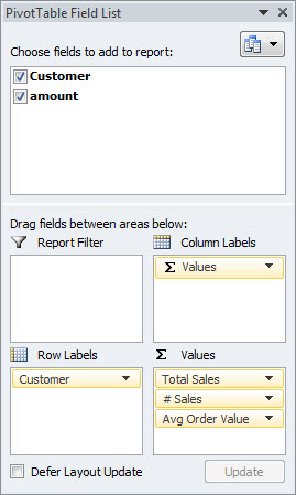
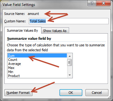
The Pivot Table headers can be overtyped so allow for more meaningful labels. The two additional picture below show the PivotTable Field Lists and the Value Field Settings dialog used to create the pivot table report. The Value Field Setting dialog is displayed with a right mouse click on the pivot table header you want to adjust. That displays a sub menu where you can select Value Field Setting. In that dialog you can decide to make the field a SUM, COUNT, AVERAGE, or various other mathematical functions. The header name can be changed here as well as the Number Format can be set for that column. Repeat for each column you want to adjust.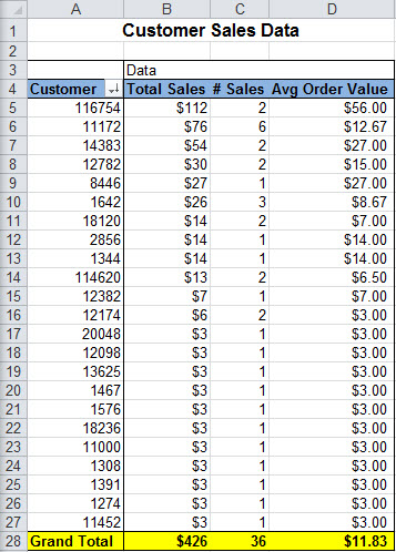
 Thanks,
Jerry
Q-28460798-customer-sales-.xls
- Total Sales is SUM of amount
- # Sales is COUNT of Customer
- Average Order is the AVERAGE of amount
The Pivot Table headers can be overtyped so allow for more meaningful labels. The two additional picture below show the PivotTable Field Lists and the Value Field Settings dialog used to create the pivot table report. The Value Field Setting dialog is displayed with a right mouse click on the pivot table header you want to adjust. That displays a sub menu where you can select Value Field Setting. In that dialog you can decide to make the field a SUM, COUNT, AVERAGE, or various other mathematical functions. The header name can be changed here as well as the Number Format can be set for that column. Repeat for each column you want to adjust.
Thanks,Jerry
Q-28460798-customer-sales-.xls
or, use SUMIF
create a list of your unique customers, perhaps below the main table
use this function
=SUMIF($A$1:$A$37,A40,$B$1
the structure is:
=sumif(Customer Range,Cell containing that customer,Amount Range).
note the $ signs to keep these ranges constant when you copy the formula.
to make a unique list, first copy the entire list to another temp sheet. Use Filter.. Advanced Filter.. and tick Unique Records Only. Copy the results back to below your main list.
and just sort the results table at the end to get your descending layout.


EARN REWARDS FOR ASKING, ANSWERING, AND MORE.
Earn free swag for participating on the platform.
Another Alternative: Insert Subtotals.
Sort the data by Customer Number and then use the Subtotal Wizard to insert subtotal rows within the data. This will also add Grouping outlines to the data. If you collapse all groups and then resort by value column, the data hidden by the collapse groups will stay with the sorted subtotal.
Thanks
Rob H
Microsoft Excel
--
Questions
--
Followers
Top Experts
Microsoft Excel topics include formulas, formatting, VBA macros and user-defined functions, and everything else related to the spreadsheet user interface, including error messages.