color/flashing cells

Is it possible that the colors of the rows will be anything other than those shown here?  That is: "Kall" is currently showing red rows; "Mig" shows pink rows.  Could there be other colors for these same values?  

Also, how many possible values might exist for the cells A8:A11?  I'm wondering if a set of conditional formatting rules could be set up if there are not too many and if the colors are mutually exclusive to the values there.

just as an example, see my modified workbook.  The colors are determined by two conditional formatting rules only; no fill colors exist.  I also used conditional formatting for C24=P24 (green if equal, regardless of value), C25-P25 (green if equal).

IMO, blinking cells are annoying and hard to set in an effective manner (ex., number of blinks, rate of blinking, colors to use).  So instead, I created another set of conditional formatting rules that greatly highlight the C and P values when not equal.  Change one to see what I mean. :-)

Also, did you want a similar coloring method applied for the lower table (rows 18:21)?

Regards,
-Glenn
EE-Sample1.xlsx

Thanks Glenn Ray for your reply,but not this what i seeking, the values in A8:A11 and N8:N11 are not pre-defined.
means I can`t know what user could put in theses cells, the point is whatever you enter into these field it should seek/match/search the value in the other side and colored it.
about the color specifically, it not a matter which to choose any color is ok (but must be the same for each vale in both tables)

I understand that the values in rows A8:A11 and N8:N11 could change.  Please remove the existing values from the example file and note that the fill colors disappear.  Then add "Kall" and/or "Mig" to ANY cell in those ranges..you'll see the row highlight automatically.

Again, if there is a limited set of values that could exist in these ranges - and you can assign a specific color for each values - conditional formatting is very effective.

Otherwise, a VBA routine would definitely be required.

Regards,
-Glenn

Hi again.
well i have tried your solution , still facing problem using conditional formatting instead of vba.
if i change "kall" value to for example "Dar" it will not seeking the value in the other side and colored it .
the values entered in the range are "Unlimited" and also can`t be defined. it could be ANY value .
it must be away to seek the value in both sides (both ranges) then colors value that matchs in same color for both range.

Okay, you helped explain the evironment much better in your latest response and that confirms that a VBA solution will be required.  It's definitely possible and I'll try to supply a solution for you this weekend.

I will say that even though VBA can produce "flashing" cells, I'm still not a proponent of them.  Does the conditional formatting on the summary cells in rows 24 aznd 25 work for you as in my example?

-Glenn

Yup seems ok in rows 24 and 25, but for learning issue If by the way you could also provide code for it  , it will be ok also :}

Okay, I'll include a limited flashing option.

thnx alot, hope you could provide solution as soon as possible.

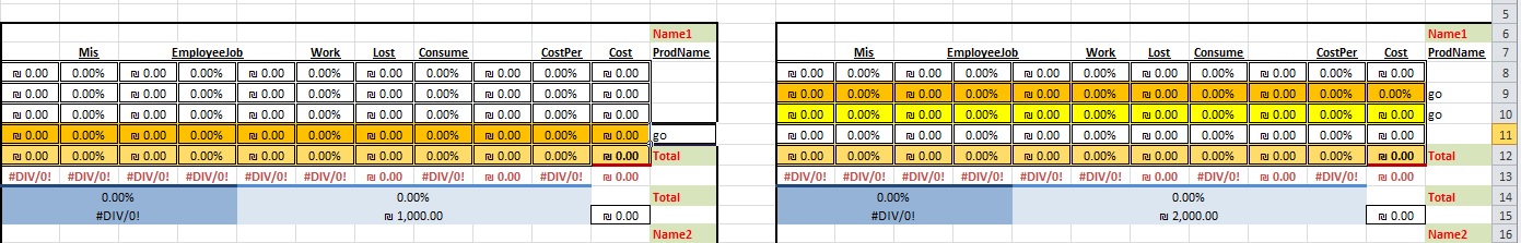
I know you want flashing...and I'll get to that later... but I did come up with a better conditional formatting system that meets your requirements.  Additionallly, you could re-define the color set that I've assigned much easier than if it was in VBA code.

Basically, if a value is in both column A or N, the rows in B:L will highlight as
Red
Orange
Yellow
Green
and the matching value's rows in O:Y will highlight as the exact same color.

Please see the example file to test.  I've also modified the colors on the bottom section (row 24 and 25) to better differentiate them from the colors on top.

If I was writing a VBA routine, it would follow similar logic seen in the conditional formatting rules.

Regards,
-Glenn
EE-Sample1.xlsx

needs fix, if in A8:A11 i put 2 same value "go" + "go" , it will not color them.
it`s only  color the left side (N8:N11)

Sorry; it works for me.  I inserted "go" in cells A9 and A10 and also in cell N11.  It highlighted the matching rows as you requested:

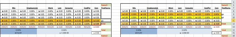
Please attach an example of your test file (my latest submission with your values).

Regards,
-Glenn

it`s not with same color, same cells value should have same colors.

Okay, here's another attempt without using VBA...I'd really like to avoid that if possible, even though a Worksheet_Change event would capture and check for value matches.

Here I've added a set of array functions to contain the list of all possible values in A8:A11 and then use conditional formatting to match against that list.  The formula in M8 is
=IFERROR(INDEX($A$8:$A$11,MATCH(0,COUNTIF($M$7:M7,$A$8:$A$11),0)),"-")
and is copied down.  M7 equals 0 and needs to remain so.  I've turned the font white so they aren't seen.

Sorry for the delay.  I hope this meets your needs.
-Glenn
EE-Sample1b.xlsx

after a check, it works!!! , thanks alot glenn ray!! I Appreciate you hard work to supply the connect solution:}}}}
I`ll be glad if you supply also a  vba code just for learning purpose (in case you have time for it)
at now this do the job.