WeThotUWasAToad
asked on
Convert report with an excessive number of rows to a more concise format in Excel
Hello,
Fig. 1 below shows the format displayed by the freeware website-platform Magento when the following report is created from the dashboard:
Reports > Products > Products Ordered
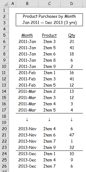
For each month, an individual row is created for each product with one or more sales. Products with no sales that month are not shown. Needless to say, this format utilizes an excessive number of rows and is therefore cumbersome to analyze and manipulate.
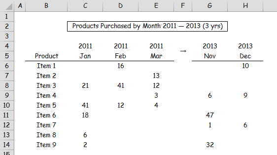
After downloading the report (as a CSV file) and saving it as an .xls file, what formula or method would be best for converting the data to the more concise table-like format shown in Fig. 2?
Thanks
PS Please provide solutions using only Excel formulas (ie without using VBA) if that is possible.
Fig. 1 below shows the format displayed by the freeware website-platform Magento when the following report is created from the dashboard:
Reports > Products > Products Ordered
For each month, an individual row is created for each product with one or more sales. Products with no sales that month are not shown. Needless to say, this format utilizes an excessive number of rows and is therefore cumbersome to analyze and manipulate.
After downloading the report (as a CSV file) and saving it as an .xls file, what formula or method would be best for converting the data to the more concise table-like format shown in Fig. 2?
Thanks
PS Please provide solutions using only Excel formulas (ie without using VBA) if that is possible.
ASKER CERTIFIED SOLUTION
membership
This solution is only available to members.
To access this solution, you must be a member of Experts Exchange.
I noticed that the data and report were in different rows and columns than your screenshots. I inserted blank rows and columns to align the worksheets to match in the attached file. As a result, the formulas will be slightly different.
=IFERROR(1/(1/SUMIFS(Sheet
=IFERROR(1/(1/SUMIFS('Alt Sheet1'!$D:$D,'Alt Sheet1'!$C:$C,$B6,'Alt Sheet1'!$B:$B,--(C$5 & " 1, " & C$4))),"")
MakePivotTableQ28489423.xlsx
=IFERROR(1/(1/SUMIFS(Sheet
=IFERROR(1/(1/SUMIFS('Alt Sheet1'!$D:$D,'Alt Sheet1'!$C:$C,$B6,'Alt Sheet1'!$B:$B,--(C$5 & " 1, " & C$4))),"")
MakePivotTableQ28489423.xlsx
ASKER
Thanks Brad. I've heard of pivot tables many times in the past but have never understood their actual function until now. Thanks for your excellent response including the detailed steps.
=IFERROR(1/(1/SUMIFS(Sheet
The above formula requires Excel 2007 or later for the SUMIFS function. It assumes that the dates in Sheet1 column A are stored as text rather than as a date time serial number that looks like text.
Should the latter assumption not be correct, then you could use a formula like:
=IFERROR(1/(1/SUMIFS('Alt Sheet1'!$C:$C,'Alt Sheet1'!$B:$B,$A5,'Alt Sheet1'!$A:$A,--(B$4 & " 1, " & B$3))),"")
The first formula is shown on worksheet Formulas, while the second is shown on worksheet Alt Formulas in the workbook attached.
MakePivotTableQ28489423.xlsx