asked on

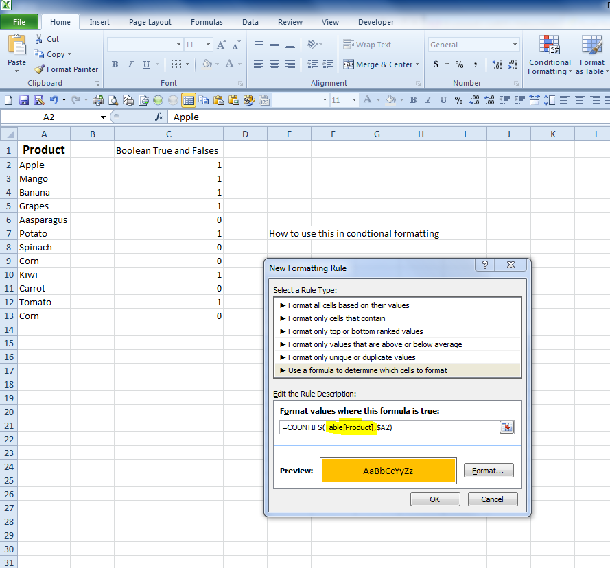
Excel Question Referring to Table Column in Condtional Formatting Formula bar

plz see the attached file.

i have two sheets that i have highlighted ListB with Conditional Formatting COUNTIFS formula and i used named range.
=COUNTIFS(Product,$A2) Product is the named range. it perfectly works.

Now, i tried this with another senario, i have two sheets and in the " ListB HighlightNEED" i want to highlighted similar to the previous senario but this time using the table column name =COUNTIFS(Table[Product],$A2) but excel does not allow me to use this. i was wondering how to refer the table column in the abovementioned formula inside condtional formatting.
Book1.xlsx

Jacques Geday

What do you mean by:
table column name =COUNTIFS(Table[Product],$A2)

Are you referring to the Table in sheet ListA Table ?

Not clear what you want to achieve if you can explain.
gowflow

Professor J

ASKER

please see the example attached. you can see that the referrence to the table works as input into the cell but when i use the same formula inside condtional formatting then it wont accept it.

Book1.xlsx

Jacques Geday

I see what you mean but still for me Table[Product] is same as Product ??? not sure !!!

anyhow I found something that maybe would help regarding Tables and conditional formatting.

http://excelsemipro.com/2011/04/excel-tables-styles-conditional-formatting-and-data-validation/

What are you after in the formula that you have ? can you clarify ?
gowflow

Professor J

ASKER

gowflow.

I do not think you understand my question at all. the link you shared is completely irrelevant to the question I asked.

perhaps the other two sheets got you confused. now I attached the workbook and I deleted the irrelevant sheets.

please look at the attached workbook. it has two sheets only. in sheet ListB range A2:A13 there is a conditional formatting and the formula used to trigger the conditional formatting is =COUNTIFS(ListA!$A$2:$A$9,$A2) and you can see it works perfectly. any value in the range A2:A13 of ListB sheet is highlighted in yellow if it exists in sheet ListA Range A2:A9. now, you can see that the ListA sheet data is in the excel table and I am sure you know how the columns of table are referenced in cells for example ListA range A2:A9 can be referenced in formulas like this Table[Product]
so, what exactly I am looking for is that the formula =COUNTIFS(ListA!$A$2:$A$9,$A2) that I currently have. I want to use the table reference instead of using "ListA!$A$2:$A$9" . you can see in the attached workbook ListB cell C2 and D2 shows the formula that I used =COUNTIFS(Table[Product],$A2) instead of =COUNTIFS(ListA!$A$2:$A$9,$A2)
and in cell it works. however, when I put the =COUNTIFS(Table[Product],$A2) into the conditional formatting then it does not accept and gives me warning that it cannot accept the table reference.
my main concern is that if the formula =COUNTIFS(Table[Product],$A2) can work in a cell, why cannot it work in the conditional formatting.

I hope this time it Is crystal clear what my goal is to achieve.

Professor J

ASKER

the attachment uploaded

ASKER CERTIFIED SOLUTION

Glenn Ray

membership

This solution is only available to members.

To access this solution, you must be a member of Experts Exchange.

Start Free Trial

Professor J

ASKER

you are Genius Glenn.

you solved the mysterious issue

Glenn Ray

Nope, not a Genius; just happened to have experienced this before you did. I was just a frustrated and surprised by the solution.

-Glenn

Professor J

ASKER

indeed you are very experienced expert in Excel. I was beating my brain against the wall trying different methods and it was not working. from what I understood, the same solution applies if faced with the data validation. right?

thank you again for saving my day