WeThotUWasAToad
asked on
Retrieving values when two variables are present in Excel
Hello,
This one's not only got me stumped but I don't even know where to begin.
In a case with a single variable (ie where a user inputs only one value), I can often find a solution using =VLOOKUP(). However, in this case, two variables are present so it will require more than what's in my bag of tricks.
Also, I have a suspicion that the format which currently exists in my spreadsheet (and is shown in the screenshots I've included) is not really conducive to the lookup process. Therefore, I suppose part of this question relates to how best to reorganize what is present into a more usable form.
As is usually the case, I'm hopeful that a solution can be provided which uses only Excel formulas and not VBA. I realize that's not always possible but if it is, that is my preference.
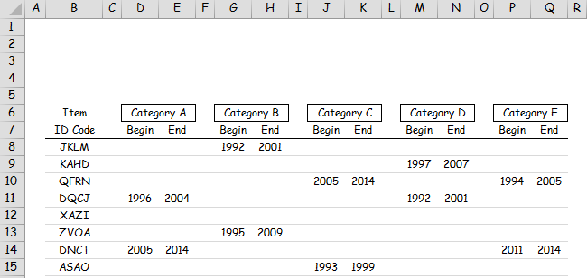
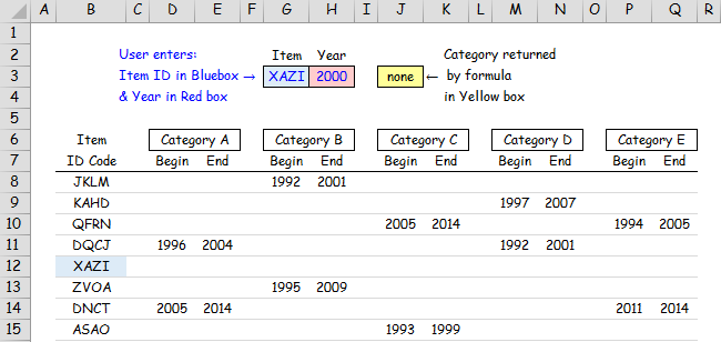
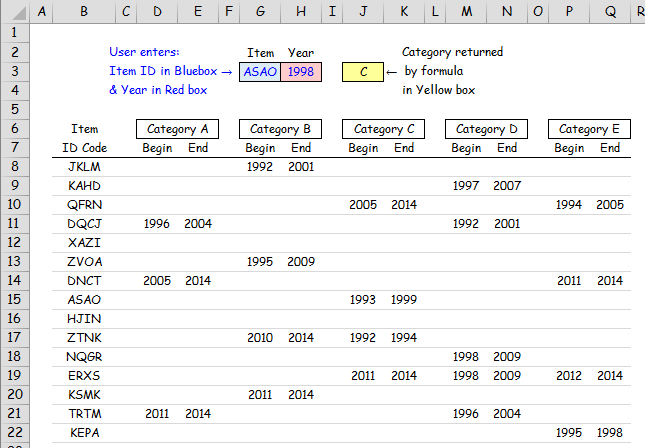
Suppose you've got a spreadsheet which contains a list of several hundred items (in column B), each of which is identified by a unique 4-character code. And suppose that for some specific period of time in the past, each item may have belonged to one or more of five categories, A thru E (Fig. 1.):
 Now suppose you designate two fields (cells), as shown in the next screenshot (Fig. 2), for a user to enter an item code (blue box) and a year (red box):
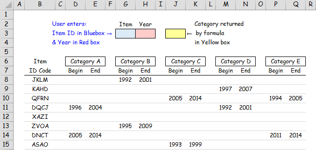 What formula in the third cell (yellow box) would display the category, if any, to which an item belonged during the year specified?
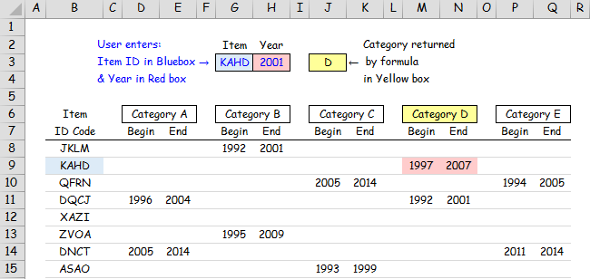
For example, say the user enters KAHD as the item number and 2001 as the year. The yellow result box should display Category D since Item KAHD belonged to that category for the time range 1997-2007 (Fig. 3).
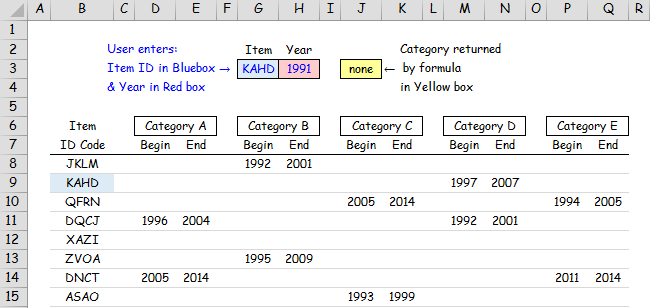
 Alternatively, suppose the user keeps the same ID code but changes the year to 1991. In that case, the yellow box should not return any category because that item was not categorized at that time (Fig. 4):
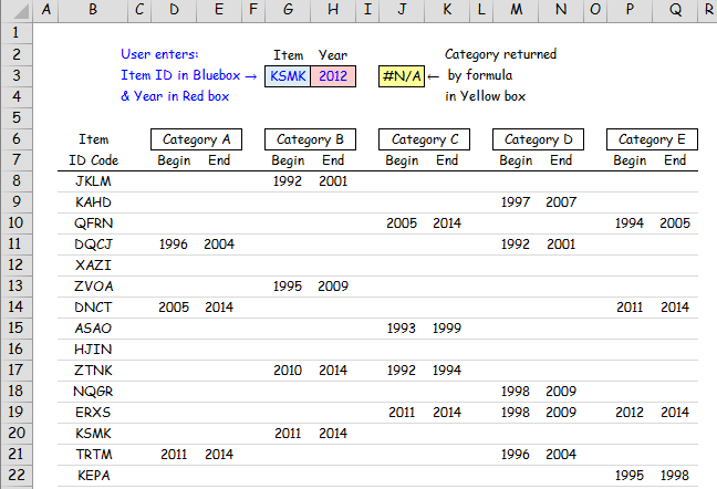
 This same result would also occur for any entered year if the item has never been categorized in a group (Fig. 5):
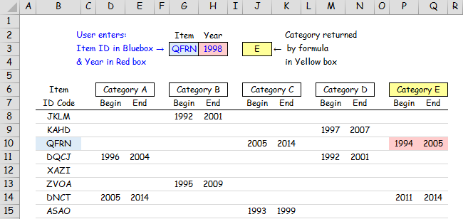
 Some items were categorized in one group for a period of time and then subsequently switched to another category. This is the case for Item QFRN where the user-entered year of 1998 would yield the result Category E (Fig. 6)
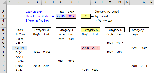
 …but changing to the year 2009 would return Category C (Fig. 7)
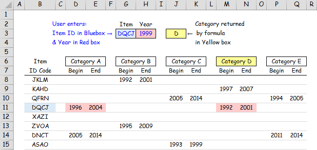
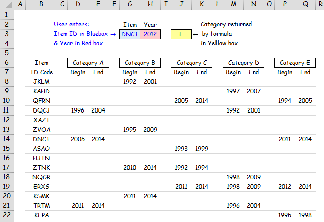
 And finally, it's possible for a given item to simultaneously be categorized in more than one group. That is the case for Item DQCJ which was in Category D for the years 1992-2001 and Category A during 1996-2004. In this case, if the user were to enter a year during the overlap (1996-2001), the result box should display the higher of the two or more categories (ie category priority is A < B < C < D < E) as shown here (Fig. 8):
 Thanks
This one's not only got me stumped but I don't even know where to begin.
In a case with a single variable (ie where a user inputs only one value), I can often find a solution using =VLOOKUP(). However, in this case, two variables are present so it will require more than what's in my bag of tricks.
Also, I have a suspicion that the format which currently exists in my spreadsheet (and is shown in the screenshots I've included) is not really conducive to the lookup process. Therefore, I suppose part of this question relates to how best to reorganize what is present into a more usable form.
As is usually the case, I'm hopeful that a solution can be provided which uses only Excel formulas and not VBA. I realize that's not always possible but if it is, that is my preference.
Suppose you've got a spreadsheet which contains a list of several hundred items (in column B), each of which is identified by a unique 4-character code. And suppose that for some specific period of time in the past, each item may have belonged to one or more of five categories, A thru E (Fig. 1.):
Now suppose you designate two fields (cells), as shown in the next screenshot (Fig. 2), for a user to enter an item code (blue box) and a year (red box):What formula in the third cell (yellow box) would display the category, if any, to which an item belonged during the year specified?For example, say the user enters KAHD as the item number and 2001 as the year. The yellow result box should display Category D since Item KAHD belonged to that category for the time range 1997-2007 (Fig. 3).
Alternatively, suppose the user keeps the same ID code but changes the year to 1991. In that case, the yellow box should not return any category because that item was not categorized at that time (Fig. 4):This same result would also occur for any entered year if the item has never been categorized in a group (Fig. 5):Some items were categorized in one group for a period of time and then subsequently switched to another category. This is the case for Item QFRN where the user-entered year of 1998 would yield the result Category E (Fig. 6)…but changing to the year 2009 would return Category C (Fig. 7)And finally, it's possible for a given item to simultaneously be categorized in more than one group. That is the case for Item DQCJ which was in Category D for the years 1992-2001 and Category A during 1996-2004. In this case, if the user were to enter a year during the overlap (1996-2001), the result box should display the higher of the two or more categories (ie category priority is A < B < C < D < E) as shown here (Fig. 8):Thanks
This would be so much easier if you were to post a workbook rather than pictures. ;)
As always, it would be better for retrieving information from a data set when that data set is in more of a data grid format. For this you would have columns for:
ID Code | Start Year | End Year | Category
I think you would then be able to use INDEX and MATCH formulas to retrieve data.
Thanks
Rob H
ID Code | Start Year | End Year | Category
I think you would then be able to use INDEX and MATCH formulas to retrieve data.
Thanks
Rob H
Here's a slight modification. This one will handle an occurrence if the item ID entered is not found in the list in column B:
=IFERROR(IF(AND(H3>=INDIRE
=IFERROR(IF(AND(H3>=INDIRE
ASKER
(Note: Flyster, this post applies only to your first response. Most of it was written earlier today before your second response — which I have not yet tested — but I decided to go ahead and post it anyway.)
"…er…um…yeah, sorta…"
or perhaps:
"yes & no"?
:)
For example, entering ASAO & 1998 worked great:
 but ZVOA & 1998 did not:
 DNCT & 2012 (overlapping years) did:
 and KSMK & 2012 (which is below the rows displayed in the earlier screenshots) did not:
"Please humor me…"Wow! This may be "humoring" for you but I am nothing short of amazed. Now I'm going to have to break down ("parse" << is that the right word?) this very long formula to figure out what it's doing. (That's not a complaint but a comment re a fun and challenging project.)
"…and see if this works…"Hmm, how shall I say this? How about:
"…er…um…yeah, sorta…"
or perhaps:
"yes & no"?
:)
For example, entering ASAO & 1998 worked great:
but ZVOA & 1998 did not:DNCT & 2012 (overlapping years) did:and KSMK & 2012 (which is below the rows displayed in the earlier screenshots) did not:
ASKER
Thanks for all the responses.
That's all the attached file is — as you will see. In other words, I created the chart and then manually entered the values I'm wanting to obtain later (ie once I get an EE solution formula(s). In fact, that's what most of the screenshots I post on EE are — since the original files commonly contain confidential contents, as is the case with this one.
So the question I guess is:
Do you want files even if they are fabricated?
c-EE-uploaded-2014-10-14.xlsx
This would be so much easier if you were to post a workbook rather than pictures. ;)Happy to oblige Rory (it's attached) but I'm curious to know (and for future threads) if your statement applies to files which have been "dry-labbed" as we…er…I mean others used to call it back in school. It means starting with what the results should be and then fabricating the equations and data, etc, backwards so they fit with the beginning conditions.
That's all the attached file is — as you will see. In other words, I created the chart and then manually entered the values I'm wanting to obtain later (ie once I get an EE solution formula(s). In fact, that's what most of the screenshots I post on EE are — since the original files commonly contain confidential contents, as is the case with this one.
So the question I guess is:
Do you want files even if they are fabricated?
c-EE-uploaded-2014-10-14.xlsx
ASKER
As always, it would be better for retrieving information from a data set when that data set is in more of a data grid format.Rob, I'm glad you mentioned this because it's something I included in my initial post:
Also, I have a suspicion that the format which currently exists in my spreadsheet (and is shown in the screenshots I've included) is not really conducive to the lookup process. Therefore, I suppose part of this question relates to how best to reorganize what is present into a more usable form.The actual data is currently arranged in the format or configuration shown in my screenshots. I recognized it to be awkward but, aside from changing it manually (which is impractical due to the large number of entries), I'm not sure how to utilize Excel formulas to effect a change.
Flyster has (remarkably) bypassed that step but rearranging is something in which I'm still interested since it will cause other future operations and formulas to be simpler.
I'm happy to post this rearranging question in a new thread if you recommend it…
…especially since, as Rory knows, I've already got all the screenshots. hehe ;)
Do you want files even if they are fabricated?
Yes. As long as they are accurately representative of your data so they can be used for developing and testing solutions. It's a lot simpler and less effort (in total) for you to create that than it is for each of us to create our own file, based on what we think you have. :)
SOLUTION
membership
This solution is only available to members.
To access this solution, you must be a member of Experts Exchange.
ASKER CERTIFIED SOLUTION
membership
This solution is only available to members.
To access this solution, you must be a member of Experts Exchange.
SOLUTION
membership
This solution is only available to members.
To access this solution, you must be a member of Experts Exchange.
ASKER
I've also added a revised layout with just 4 columns on a new tab which makes the formulas a lot simpler!Thanks Rory, that is a lot simpler — but…
How did you do it or what steps/formulas did you use?
In other words, did you just move things around manually by copy/pasting, etc or did you use formulas in some way?
Most importantly, could you have rearranged the data in the same way if the spreadsheet had a few thousand rows rather than the 15 or so in the demo?
Thanks
ASKER
This formula should fix the above mentioned errorsThanks Flyster, yes it did fix the errors and now works great.
Thanks also for the explanation. That's very helpful along with arranging your formula as shown below so it's easier to follow. I'm pasting it here in that form only for my own future reference:
=IFERROR(
        IF(AND(H3>=INDIRECT("P"&MATCH(G3,B8:B22,0)+7),H3<=INDIRECT("Q"&MATCH(G3,B8:B22,0)+7)),"E",
        IF(AND(H3>=INDIRECT("M"&MATCH(G3,B8:B22,0)+7),H3<=INDIRECT("N"&MATCH(G3,B8:B22,0)+7)),"D",
        IF(AND(H3>=INDIRECT("J"&MATCH(G3,B8:B22,0)+7),H3<=INDIRECT("K"&MATCH(G3,B8:B22,0)+7)),"C",
        IF(AND(H3>=INDIRECT("G"&MATCH(G3,B8:B22,0)+7),H3<=INDIRECT("H"&MATCH(G3,B8:B22,0)+7)),"B",
        IF(AND(H3>=INDIRECT("D"&MATCH(G3,B8:B22,0)+7),H3<=INDIRECT("E"&MATCH(G3,B8:B22,0)+7)),"A",
        "None"))))),
"None")
I did it by hand as it was a small data set. For bigger data I would code it.
ASKER
Thanks for the solutions.
=IF(AND(H3>=INDIRECT("P"&M
Flyster