Excel Pivot Table - Running total that doesn't end at 100%

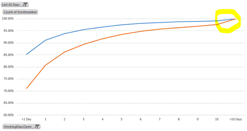
I've got a dataset in Excel for which I want to display the running total. However, I want the display to end before I get to 100% - see the below image:


The right-most data element is for tickets open longer than 10 days (">10 Days"), but I don't want to include that particular value in the display chart, but instead have the chart end at 10 days and the lines end at 96% (or whatever they would end). The problem I'm having is that, when I uncheck the ">10 Days" data element in my pivot table to remove it from display, Excel re-calculates the running total so that the remaining data elements still add up to 100%.

In essence, I guess I'm looking for Excel to calculate the running total as a total of all data in the set, not just what I've chosen to display. If I uncheck items in the pivot table, I want them hidden from display but I want their values still included for the purpose of the summary.

Does that make sense? Is it possible? My initial research tells me it's not, and I'd considered formatting the pivot table properly, copying my data into a new static table and building a standard chart based on that instead. If I can do it inside the pivot chart so that it stays connected, that's ideal though.

If it matters, I'm using Excel 2013.