holemania
asked on
Excel - Array Vlookup
I have an excel spreadsheet with one worksheet called "Material" and another worksheet called "Reference". Based of values from "Material" worksheet, it would look at the "Reference" worksheet to see which chart to use and what the "Polishing Lb" is. Is it even possible to use formulas to do an array vlookup?
In this example, my worksheet "Material" has all these columns with values. The "Polishing LB" is what I am trying to do a lookup against.
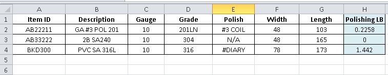
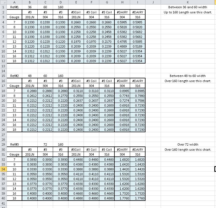
So the 3 charts is based of the Width and Length, on which chart to use.
Once the chart is determine than the Gauge, Grade, and Polish is what determine the Polishing LB. Is it even possible to do this lookup by formula, or would a VBA script be necessary. Can someon provide sample?
Also attaching the excel.
STEEL---POLISH-CHART.xlsm
In this example, my worksheet "Material" has all these columns with values. The "Polishing LB" is what I am trying to do a lookup against.
So the 3 charts is based of the Width and Length, on which chart to use.
Chart 1 - Width is between 36 and 60, and length is up to 160.
Chart 2 - Width is between 48 to 60, and length is over 160.
Chart 3 - Width is over 72 and length is over 160.
Once the chart is determine than the Gauge, Grade, and Polish is what determine the Polishing LB. Is it even possible to do this lookup by formula, or would a VBA script be necessary. Can someon provide sample?
Also attaching the excel.
STEEL---POLISH-CHART.xlsm
ASKER CERTIFIED SOLUTION
membership
This solution is only available to members.
To access this solution, you must be a member of Experts Exchange.
SOLUTION
membership
This solution is only available to members.
To access this solution, you must be a member of Experts Exchange.
SOLUTION
membership
This solution is only available to members.
To access this solution, you must be a member of Experts Exchange.
Saqib Husain
File?
thanks Syed
STEEL---POLISH-CHART2.xlsm
STEEL---POLISH-CHART2.xlsm
ASKER
Thanks all. I will take a look at each propose solution. The "N/A", if there's nothing I want to show a zero.
ASKER
Thanks all. I had tried all 3 and all 3 worked well. Rory's solution was probably the easiest for me to follow and will use his solution, but will divide points amongst all 3. However, I do have a question to Rory. If it's N/A, can the formula be tweaked to show a zero instead?
Will the N/A only ever appear in one column, or could it be in any of the three criteria columns?
ASKER
As far as I can tell, it's only in the Polish column. However, if it's not able to find the value, I also want to list as zero. So I guess it would not matter which column, long as it can't find a match, it would show 0 instead of N/A as the result.
In that case:
=IFERROR(INDEX(CHOOSE(I2,r
still array-entered using Ctrl+Shift+Enter.
=IFERROR(INDEX(CHOOSE(I2,r
still array-entered using Ctrl+Shift+Enter.
ASKER
Thanks.