StevenPMoffat
asked on
Sum up values on Row in Excel based on comparison to values in headers.
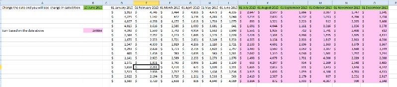
I would like to be able to sum up the values in a row, where the values that I include are based on comparing the header values to a set value, a date for instance. In this case, I want to sum all the values in the various columns wherein the column heading (a date) is later than a fixed value. As that fixed value changes, the summation will adjust accordingly.
aikimark
Please post a sample workbook
in general, you probably can use the SUMIF / SUMIFS formula in this case, but as mentioned, try post a sample file so to make things easier.
@StevenPMoffat
please see attached. were you looking for solution like this?
formula
please see attached. were you looking for solution like this?

formula
=SUMPRODUCT(--($D$1:$O$1>=$B$1)*($D$2:$O$17))ASKER
Getting closer. I updated the file as I want the SumProduct to be row specific. I also want the matrix in a table. In this example, it seems to be skipping the data in Columns H,I,K??? When I zero them out, the sum doesn't change.
Also what is the purpose of the "--" in the formula do?
Also would be nice if the formula could refer to the table header row as opposed to absolute cell references like $D$1:$O$1, but when I do that, the sums come back 0.
Book2.xlsx
Also what is the purpose of the "--" in the formula do?
Also would be nice if the formula could refer to the table header row as opposed to absolute cell references like $D$1:$O$1, but when I do that, the sums come back 0.
Book2.xlsx
ASKER
Sorry. Thought I had posted the original sample file to work with. Here it is.
no file
Hi Steven,
please find attached. i have fixed the formula based on your latest requirement.
the formula uses now table header and does the calculation based on the row
double negative forces formula to return the TRUE and FALSE to 0s and 1s it is simple a math operation. if we change the double negative to +0 or *1 it would still do the job. i usually use double negative which is the same as +0 or *1
=SUMPRODUCT(--(Table1[#Headers]>=$B$1)*(Table1[@]))ASKER
Sorry, I wish the original example file was loaded. Not sure why I can't get it loaded, but when I applied your concept to my real data file, I am getting some errors. I believe it is because I want the formula to be part of the table (one of the columns) and the references you use for #Headers and [@] get confused and introduce a circular reference. All I am getting is 0s. See attached file for latest incarnation. Is there any other way to reference the table headers and the rest of the columns without including the first or previous columns?
Book4.xlsx
Book4.xlsx
This version of the formula gets rid of the circular references.
=SUMPRODUCT(--(Test!$D$23:$W$23>=$G$17)*(Test!$D24:$W24))ASKER
Is there a way to do this without having to refer to specific cell locations and use some sort of table reference? LIke
=SUMPRODUCT(--(Planning2[[
There is no circular references, but for some reason it doesn't matter what is in cell G17.
=SUMPRODUCT(--(Planning2[[
There is no circular references, but for some reason it doesn't matter what is in cell G17.
You could name the range of date headers.
Steven,
please find attached. =SUMPRODUCT(--(Planning2[[
Book4.xlsx
please find attached. =SUMPRODUCT(--(Planning2[[
Book4.xlsx
ASKER
Professor. It doesn't seem to be working.
With the file you sent me, with a date of 12/11/2015 in G17, the first row should only sum up to 32 and not 64. 64 is the entire row, with 32 in the column with date of 11/27/2015.
With the file you sent me, with a date of 12/11/2015 in G17, the first row should only sum up to 32 and not 64. 64 is the entire row, with 32 in the column with date of 11/27/2015.
Steven, i got a bit confused here, so excuse me.
isn't the criteria just the dates or the number of cells? becuase lets say, your date is 12 november 2015 and then the values in the row 24 , one of them is unser 27 november and the other one is under 25 december, meaning that both of these dates are greater then the G17 hence it is counting it. why should it not count it then? can you please elaborate?
isn't the criteria just the dates or the number of cells? becuase lets say, your date is 12 november 2015 and then the values in the row 24 , one of them is unser 27 november and the other one is under 25 december, meaning that both of these dates are greater then the G17 hence it is counting it. why should it not count it then? can you please elaborate?
ASKER
Put in a date of 12/11/2015 in G17 and the value under 11/27/2015 shouldn't be summed up, but it is. I can tell, because if I zero out the value under 11/27/2015 the total changes.
I might suspect that the values inside the square brackets are being interpreted incorrectly as numeric values and not as date values that match column headers.
Steve,
can you please elaborate why the value under 11/27/2015 should not be counted?
as we can see that this amount under 11/27/2015 should be excluded becuase the date 11/27/2015 is greater than the date of 12/11/2015 Correct?
if value udder as per your statement need to be excluded then what is exactly the criteria? in cell G17
ASKER
The date of 11/27/2015 is actually less than 12/11/2015 and not greater than as you just posted. Therefore, it shouldn't be counted, but it is???
ASKER CERTIFIED SOLUTION
membership
This solution is only available to members.
To access this solution, you must be a member of Experts Exchange.
ASKER
Thanks for persevering with me.
you are most welcome Steven, i am glad i was able to help