Problem to calculate

You like to have a Alphabetic value in one of the Cells.

I was able to reproduce the #VALUE! error by entering 22/1/16 as text (by prefixing with a single quote) and in the other a real date formatted d/m/yyyy. In my American Windows, the short date default format is m/d/yy so Excel got confused by the 22 in the first position.

If I change the text date to one that looks valid to an American (e.g. '1/12/16) then the results of the calculation are displayed correctly because Excel converts the text date into a real date time serial number before performing the subtraction.

If the above discussion does not explain your problem, please post a sample workbook that reproduces the problem.

See if those dates have the correct date separator depending on your regional settings.

Both dates are "Date" cell having the format like

14.12.2015 14:45

Select allOpen in new window

I still get the same problem, using this

=DATEVALUE(TEXT(L2,"DD/MM/YYYY hh:mm:ss"))-DATEVALUE(TEXT(I2,"DD/MM/YYYY hh:mm:ss"))

Select allOpen in new window

Error could also be caused by:
1) Format error: Subtracting 2 dates may yield a NEGATIVE result (if value to be subtracted is larger)
2) Insufficient column width: Result may exceed column capacity; enlarge the column width
3) Wrong data type of result: Try formatting the result cell as just a plain number

Really L2 is bigger than I2.

I also get the same problem to this

=+(DATEVALUE(TEXT(L2,"DD/MM/YYYY hh:mm:ss"))-DATEVALUE(TEXT(I2,"DD/MM/YYYY hh:mm:ss")))

Select allOpen in new window

This =DATEVALUE(TEXT(L2,"DD/MM/YYYY hh:mm:ss")) itself is throwing the error. It is not converted.

You need get the conversion successful first to proceed.

I could get the date converted using this. See if it helps.

=DATE(MID(L2,7,4),MID(L2,4,2),LEFT(L2,2)) + TIME(MID(L2,12,2),RIGHT(L2,2),0)

Select allOpen in new window

As there can be sometimes only Date part to the cell (without time part), I still get

#NAME?

Select allOpen in new window

using this

=DATE(MID(L2,7,4),MID(L2,4,2),LEFT(L2,2))+lf(LEN(L2)>10,TIME(MID(L2,12,2),RIGHT(L2,2),0),TIME(23,59,0))

Select allOpen in new window

Change both cell number formats to "Number" to check if both values are numerical behind.
If one of them doesn't convert to a number, you may try to rewrite it manually to check if it solves.
If it solves, that may mean
1-You missed order of day, month and year.
2-Or you may entered a date that doesn't exists, such as 30th of February. =EOMONTH(,) function may help about this.
3-Or you may have a text character in cell like empty space.
4-Or you may just need to re-evaluate values. You can use text-to-columns tool (de-select all sperator characters when using) for quickly re-evaluate cells. (There is a bug here that sometimes causes Excel to crash, make sure to save before. And it is better to try on a range that doesn't have Autofilter turned on)

But original 2 cells (I and J columns) should be Date fields.

How to correct the syntax to the codes I showed?

Just change Number format to "Number" to find where error comes from as i wrote before.

You could save a lot of irrelevant guess work by uploading a sample file with only the data in question. You can delete all other information.

Can you please refer to this?
test.xls

In P2, the following formula works...

=DATE(MID(L2,7,4),MID(L2,4,2),LEFT(L2,2))+IF(LEN(L2)>10,TIME(MID(L2,12,2),RIGHT(L2,2),0),TIME(23,59,0))

Select allOpen in new window

Many thanks.

How to show how many hours this

=DATE(MID(L2,7,4),MID(L2,4,2),LEFT(L2,2))+IF(LEN(L2)>10,TIME(MID(L2,12,2),RIGHT(L2,2),0),TIME(23,59,0))-(DATE(MID(I2,7,4),MID(I2,4,2),LEFT(I2,2))+IF(LEN(I2)>

Select allOpen in new window

contains?

Your formula has LF instead of IF which is why it gave the #Name error

Can you please show with more details?

Or you may also try this.....

=TEXT(DATE(MID(L2,7,4),MID(L2,4,2),LEFT(L2,2))+IF(LEN(L2)>10,TIME(MID(L2,12,2),RIGHT(L2,2),0),TIME(23,59,0))-(DATE(MID(I2,7,4),MID(I2,4,2),LEFT(I2,2))+IF(LEN(I2)>10,TIME(MID(I2,12,2),RIGHT(I2,2),0),TIME(23,59,0))),"hh:mm")

Select allOpen in new window

BTW, is there a way to concurrently run one command, right on the cell's formula?

Did you try the formula from post#41430925?

Yes.

BTW, is there a way to concurrently run one command, right on the cell's formula?

I am failing to understand what you mean by

concurrently run one command, right on the cell's formula

When I column is

22.01.2016 10:30

L column is

24.01.2016 16:32

I do not know why I get

6:02

by this

=DATE(MID(L5,7,4),MID(L5,4,2),LEFT(L5,2))+IF(LEN(L5)>10,TIME(MID(L5,12,2),RIGHT(L5,2),0),TIME(23,59,0))-(DATE(MID(I5,7,4),MID(I5,4,2),LEFT(I5,2))+IF(LEN(I5)>10,TIME(MID(I5,12,2),RIGHT(I5,2),0),TIME(23,59,0)))

Select allOpen in new window

Can you please see this? Thanks
test.xls

Follow the procedure I have detailed above

Can you please refer to my current file?

You just need to change the "." to "/" and use the formula =K2-L2 or =I2-L2. whichever column you want to calculate the differences

To change the dots, select column I, K and L press ctrl + F. Click on Replace tab.



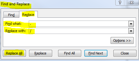
Please see attached file.
test--v2-.xls

Saqib,

I do not see your current file is fine.

Did you see my previous Excel file, inside which I did not get the time deducted in hours properly?

Excel Amusant,

Can you please refer to the last Excel file I attached yesterday, to help, as I see your current attached file is different from mine?

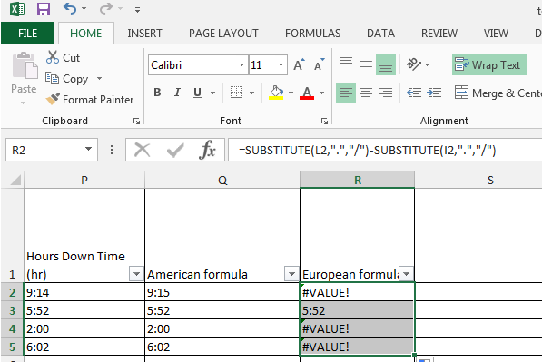
In my computer using American style m/d/yyyy dates, I got the difference of K2 & L2 using:
=SUBSTITUTE(MID(L2,4,3) & LEFT(L2,3) & MID(L2,7,20),".","/")-SUBSTITUTE(MID(K2,4,3) & LEFT(K2,3) & MID(K2,7,20),".","/")

If your computer uses European style d/m/yyyy dates, I think you may be able to simplify the formula to:
=SUBSTITUTE(L2,".","/")-SUBSTITUTE(K2,".","/")

I put both formulas in columns M & N of the Test file.

With both formulas, I used a Custom number format of:
d \d\a\y\s h:mm;@
This will display the difference like 0 days 9:38

Brad
DateTimeTestQ28919984.xls

Could you please refer to current attached file, and use the same date format as in Column I and J?

Right now, Row 5 should be wrong in Column P. How to correct it?

HuaMinChen,
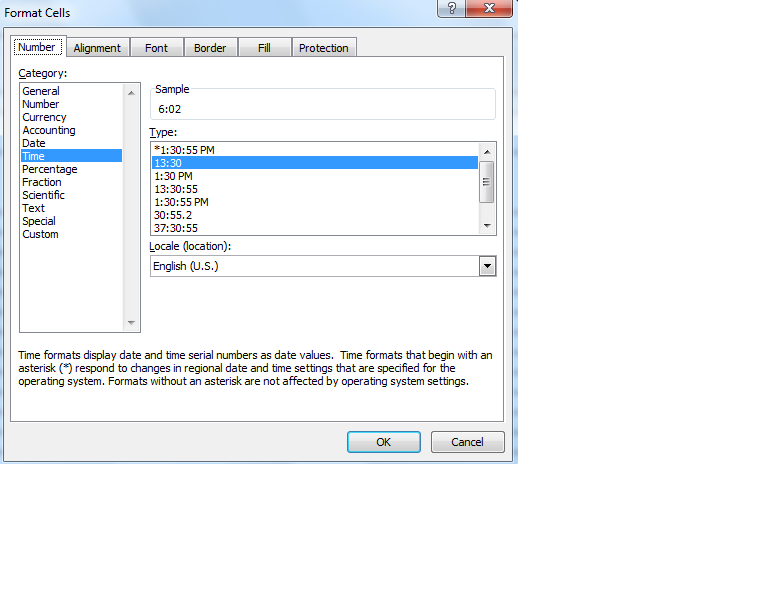
I copied the formatting from column P and applied it to columns M and N. If you prefer the format from column I and J, please copy that format and paste it in columns M and N.

I show two different formulas in column M and N. In my American format computer, column M results agree with the formulas in column P--and none of the rows show #VALUE! error.

If you see an error value in column M, does column N show the correct answer? If so, that's the formula that you should be using in column P.

Brad
DateTimeTestQ28919984.xls

Sorry, I did not put the Excel file properly. Can you please refer to it now?

Right now, Row 5 should be wrong in Column P. How to correct it?
test2.xls

HuaMinChen,
Here is a screenshot of what I see:

I cannot tell what you see in your computer in Hong Kong. Could you please post a screenshot of the attached workbook?

You most likely are running a different default date format than I am. That's why your column P shows errors and mine does not. If I were to guess, when you open the workbook attached to this Comment, you may see errors in column P & Q, but not in R. If so, please use the formula in column R.

Brad
test2Q28919984.xls

I get "6.02" in P5 and this is the problem.

P column is depending on I and J column. I only need to resolve the problem in P5 now.

Sorry Saqib, what to adjust below?

Sorry, please disregard my last message.