VBA help with macro to create pivot and group rows then move to column

Edward,
Why delete the pivot?  Why not create a different macro to just refresh the existing pivot?

I am good with that. What ever I can get working is fine with me. :)

My problem with this whole thing is that I have 8000 plus rows that I need to group to days then move to columns. I have a nice VBA script for my monthly pivot but it wont work on my weekly.

I see, so if I were to do this manually, this is what it would look like, right?  


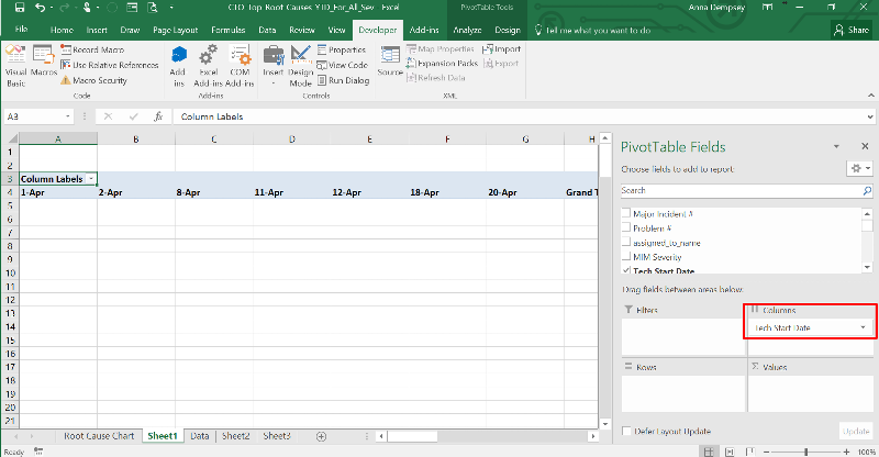
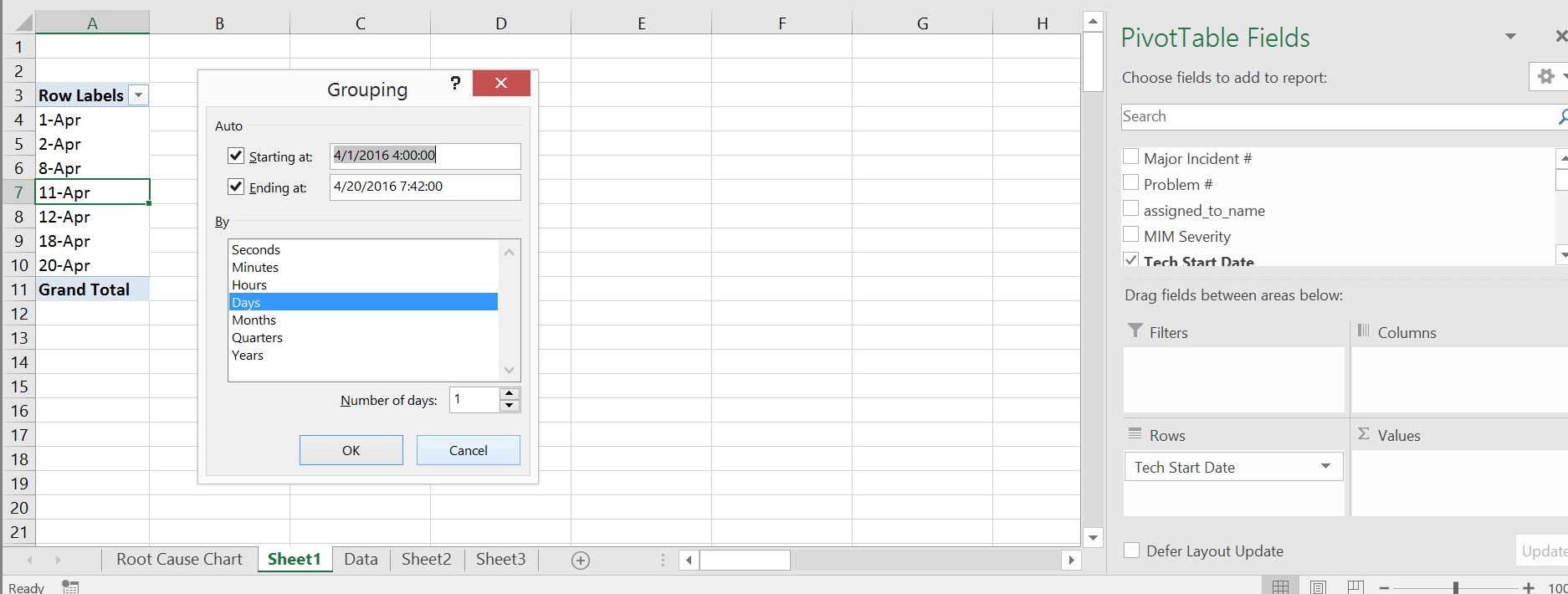
1) Group by Days


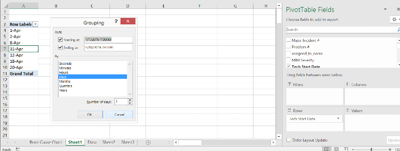
2) Move field from Rows to Columns within the Pivot Table


Is this macro only supposed to work with PivotTable7 or should it be able to work on any other pivot?

I recorded what I did in the macro. On my data sheet I have a column called weekending, in another column 8 week trend and what the 8 week trend does tells me what ticket was closed within 8 weeks and gives me the word valid at the end if it is within 8 weeks. So I drag 8 week trend to the top left (and select only valid)as a filter, drag weekending down to rows then group them to days, then drag that to column. Drag "assigned to" down to rows, then drag number down to value on the bottom right and there is my pivot.

Edward,
I am assuming the reason you need to group your dates by "DAY" is that each date contains a TIME value so you are seeing multiple rows with the same date but different times.   Then Grouping them consolidates them into a single day value.
02/20/2016 11:52 AM    - which is the number 42476.3370
02/20/2016 09:07 PM    - which is the number 42483.2020
May I suggest adding a helper column to your data and truncate the time value from the "WeekEnding" dates.  This will leave you with a column you can use in the Columns box of the Pivot Wizard that is a pure date that does not need to be grouped by day.     =TRUNC( D2),  assuming the "WeekEnding" dates are in column D.

As Jeremy suggested... Now you can build your pivot table once and just have code to refresh it whenever you have new data. The code below will refresh all pivot tables in the workbook:

Sub RefreshPivotCache()
    Dim pc As PivotCache
    For Each pc In ActiveWorkbook.PivotCaches
      pc.Refresh
    Next pc
End Sub

Select allOpen in new window

OR... if you only want to update Pivot Table 7 then try this one:

Sub UpdatePivot7()
    ActiveSheet.PivotTables("PivotTable7").PivotCache.Refresh
End Sub

Select allOpen in new window

The problem with me making this pivot table is, if I put the dates to the column, I get an error that its over 8000 columns, so what I do is put them in the rows first then group them by days and then move them back to columns.

@Jeremy, yes it looks like that after grouping, but before that I have 11000+ rows of dates, that's why I have to group them before moving them to the columns.

Edward,
Will you please post a couple of example values that are in the column of data that you are grouping by days.  Not rows of data, just a couple of the date values that being grouped.  Pure dates will group together in Pivot Table rows or columns so that is why I suggested a helper column to simplify the dates to avoid having to rebuild the pivot every time.

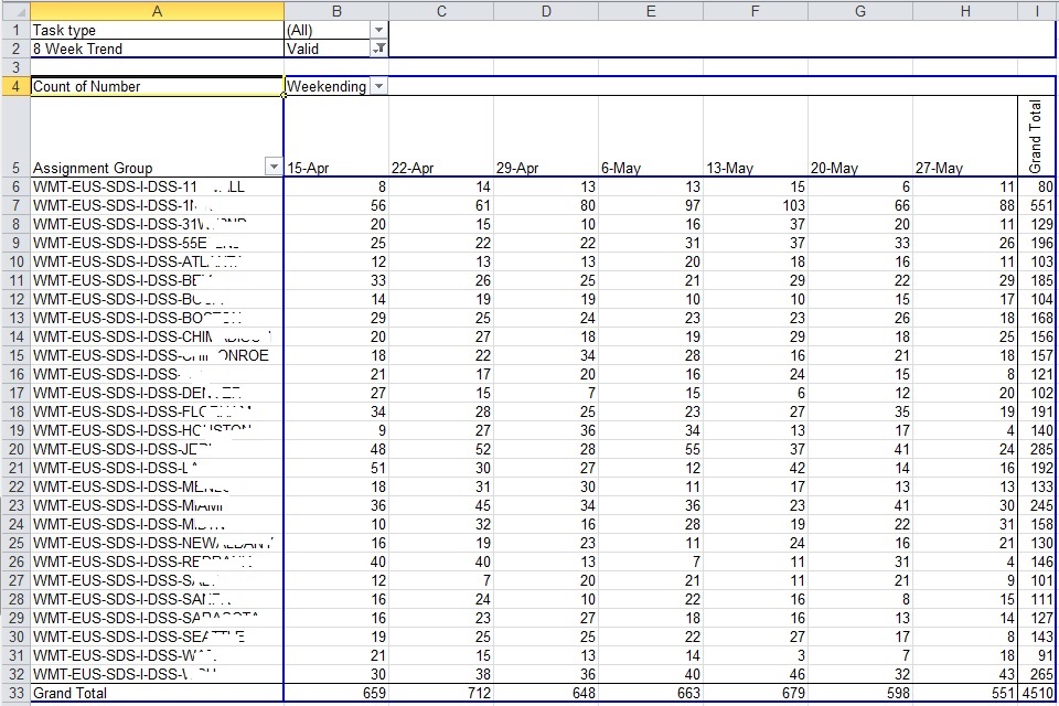
I did post the values up above of what I pivot. As for the dates they are the weekending, meaning Friday of every week during the year. For example, this month the dates would be 5/6, 5,13, 5/20, 5/27.

for the report filter, I have my 8 week trend formula column, for my column labels I have Weekending formula column, for Row labels I have assignment group, and for values I have the ticket numbers.

my 8 week trend formula is this

if(r2<today()-49,"","Valid")    <-- with this, I filter the valid which gives me all the tickets closed in an 8 week period.

The only thing is I have over 8000 rows of weekending so I cannot group them in the column section, I have to put them in the rows, group them by day then move them to column section.

I formatted the cell without the time for my weekending column.

Formatting does not change the underlying data.  Only how it appears in the cell.  Have you tried using TRUNC to strip off the decimals in the source data?

Thats not my issues. The issue is I have more than 8000 rows of data, and I cannot put that in the column area of a pivot until its grouped by days.

@Jerry, I was talking to my excel guru, and he mentioned to add Trunc to my weekending formula. And that fixed me. So I opened your sample file and I saw  you added that to my weekending formula. I wish I would have looked at that sooner. :(

Thanks this worked great!

No problem Edward.  I'm happy that we found a good solution for you.  All the best.