asked on

Excel: Counting Number of Orders / Grouping by Months

Dear Experts

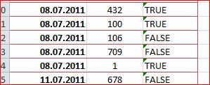
I have a table with all orders, dating back to 2011.

I would like to show the top five months since 2011 on my dashboard page.

The table also has a column with TRUE/FALSE. If the value is true, then the data is relevant for the statistics/top 5.

What is the best approach: with VBA or by using PivotTables or both?
If I were to group the orders with a pivot table, I'd need to be able to pick the top months.

I've attached a sample worksheet. Once I know how to do it, I should be able to adapt it with other tables.

Thank you for your help.
SampleData.xlsm

Professor J

Follow these steps. first if you want to see only for 2011 then filter out others and leave 2011 only.

Click on C3 on your pivot table sheet, then put the filter on. then click on Filtered header of B3 and on the dropdown select "Number Filters" then from the Dropdown select Top 10 numbers, , then a small box will appear. then reduce from 10 to 5 and click ok.

please see attached file.
SampleData.xlsm

Massimo Scola

ASKER

OK that makes sense.

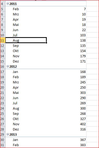
The way it is set up now, it shows the top five of every year.
How do I set it up so that it displays the top 5 months since the beginning so that it would look something likes this:

November 2013
December 2012
Januar 2014 etc..

Professor J

just fill in all dates.

click on the pivot table then go to Design then on Layout select Report Layout and on the dropdown select Repeat all items.

then repeat again the filter option as Click on C3 on your pivot table sheet, then put the filter on. then click on Filtered header of B3 and on the dropdown select "Number Filters" then from the Dropdown select Top 10 numbers, , then a small box will appear. then reduce from 10 to 5 and click ok.
SampleData.xlsm

Ryan Chong

alternatively, you can try use a Database Query (.dqy) File

For example, you can create a test.dqy file with the following content:

XLODBC
1
DSN=Excel Files;DBQ=C:\pathToYourSample\SampleData.xlsm;DefaultDir=C:\pathToYourSample;DriverId=1046;MaxBufferSize=2048;PageTimeout=5;
SELECT top 5 Year(`Orders$`.Date) as YYYY, Month(`Orders$`.Date) as M, Count(`Orders$`.CustomerID) as CustomerCnt FROM `Orders$` `Orders$` Where `Orders$`.Relevant = 1 and Year(`Orders$`.Date) = 2016 Group By Year(`Orders$`.Date), Month(`Orders$`.Date) union SELECT top 5 Year(`Orders$`.Date) as YYYY, Month(`Orders$`.Date) as M, Count(`Orders$`.CustomerID) as CustomerCnt FROM `Orders$` `Orders$` Where `Orders$`.Relevant = 1 and Year(`Orders$`.Date) = 2015 Group By Year(`Orders$`.Date), Month(`Orders$`.Date) union SELECT top 5 Year(`Orders$`.Date) as YYYY, Month(`Orders$`.Date) as M, Count(`Orders$`.CustomerID) as CustomerCnt FROM `Orders$` `Orders$` Where `Orders$`.Relevant = 1 and Year(`Orders$`.Date) = 2014 Group By Year(`Orders$`.Date), Month(`Orders$`.Date) union SELECT top 5 Year(`Orders$`.Date) as YYYY, Month(`Orders$`.Date) as M, Count(`Orders$`.CustomerID) as CustomerCnt FROM `Orders$` `Orders$` Where `Orders$`.Relevant = 1 and Year(`Orders$`.Date) = 2013 Group By Year(`Orders$`.Date), Month(`Orders$`.Date) union SELECT top 5 Year(`Orders$`.Date) as YYYY, Month(`Orders$`.Date) as M, Count(`Orders$`.CustomerID) as CustomerCnt FROM `Orders$` `Orders$` Where `Orders$`.Relevant = 1 and Year(`Orders$`.Date) = 2012 Group By Year(`Orders$`.Date), Month(`Orders$`.Date) union SELECT top 5 Year(`Orders$`.Date) as YYYY, Month(`Orders$`.Date) as M, Count(`Orders$`.CustomerID) as CustomerCnt FROM `Orders$` `Orders$` Where `Orders$`.Relevant = 1 and Year(`Orders$`.Date) = 2011 Group By Year(`Orders$`.Date), Month(`Orders$`.Date) Order By 1, 3 desc

Date	CustomerID	Relevant

Open in new window

and then double click the file to generate the result based on the SQL statement in your .dqy file.

try customize the codes accordingly.

more info:
XL97: New Database Query (.dqy) File Format
https://support.microsoft.com/en-us/kb/164729

Use Microsoft Query to retrieve external data
https://support.office.com/en-us/article/Use-Microsoft-Query-to-retrieve-external-data-42a2ea18-44d9-40b3-9c38-4c62f252da2e?ui=en-US&rs=en-US&ad=US&fromAR=1

Massimo Scola

ASKER

Thanks ProfessorJimJam

Ryan: How would I put this into cells?
Will it automatically populate five cells/rows?

ASKER CERTIFIED SOLUTION

Ryan Chong

membership

This solution is only available to members.

To access this solution, you must be a member of Experts Exchange.

Start Free Trial

SOLUTION

Jerry Paladino

membership

This solution is only available to members.

To access this solution, you must be a member of Experts Exchange.

Start Free Trial

Massimo Scola

ASKER

Ryan: So at the end, I end up having two files? The workbook and the query file.
The thing is that a number of people have access to the file. I would need to instruct every user to click on the query file first?

Ryan Chong

yup, by using a Database Query (.dqy) File, it will generate the output as another file.

but user can directly go and run the .dgy file and no need to have interaction with your source file.

Massimo Scola

ASKER

Sorry for my late reply.
I was able to implement it with the pivot table.

Please close this topic the normal way.

Thanks

Professor J

Thanks mscola for your feedback

You can close the question yourself . Simply click on whatever solution helped you and click next and close.