Excel macro to print selection
Hi Experts,
I have a program that hides rows and columns to show just what info I need.
I now need to print this filtered data.
I would like to Select the the data table then prompt to ask how many copies do you want printed.
Is there a way to force the printer properties to "print selection" AND BEST FIT TO SHEET?? Hmmmmmm
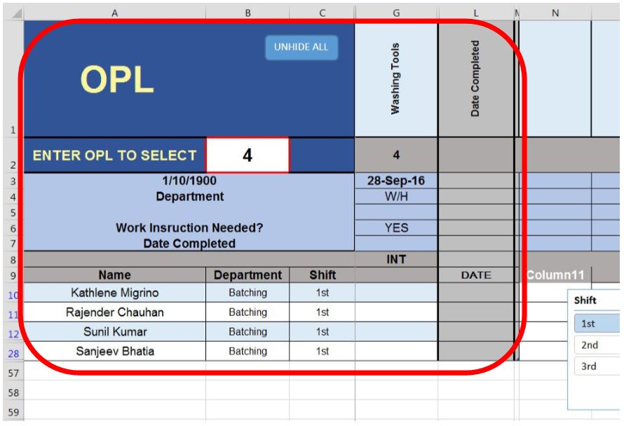
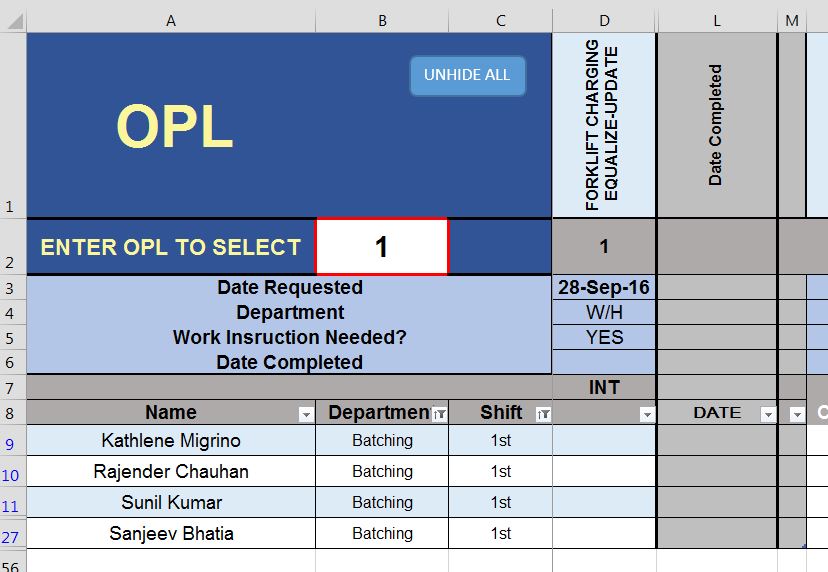
This sample image shows Column L and Column M as being the last two columns to include in the range to print, but, the table will grow and more columns will be added as I add more trainings. So the solution should be easy for me to change the LAST two grey columns later. The last row to include in the selection will always be the last name in the list.
 Thanks so much.
OPL-MATRIX.xlsm
I have a program that hides rows and columns to show just what info I need.
I now need to print this filtered data.
I would like to Select the the data table then prompt to ask how many copies do you want printed.
Is there a way to force the printer properties to "print selection" AND BEST FIT TO SHEET?? Hmmmmmm
This sample image shows Column L and Column M as being the last two columns to include in the range to print, but, the table will grow and more columns will be added as I add more trainings. So the solution should be easy for me to change the LAST two grey columns later. The last row to include in the selection will always be the last name in the list.
 Thanks so much.
OPL-MATRIX.xlsm
ASKER
Hi Rob
This range will always change everytime we select a new column to show.
I need a code that will know where the last column is and the last row to select and print.
This range will always change everytime we select a new column to show.
I need a code that will know where the last column is and the last row to select and print.
I can't download your file to implement in your file but just done so in a file of my own.
I have assumed report sheet is called OPL and then used this formula to create a Named Range "DynamicPrint":
=OFFSET(OPL!$A$1,0,0,COUNT
You may have to adjust the result of the COUNTA bits to allow for blank columns/rows in the header area; looks like A5 is blank so that would be +1 to rows (first COUNTA) and looks like columns B & C are blank so would be +2 to columns (second COUNTA).
Manually set the Print Area to something to create the Print_Area name in the Name Manager. Select the Print_Area in the Name Manager and the refers to box at the bottom will show the manual range you set. Change that to =DynamicPrint (or whatever you decide to call it).
ASKER
In the example above the last column is M and the last row is 28.
L and M are my Date columns I want to show up beside the selected row to view,.
L and M will get bumped further down when I add more and more columns (training names)
L and M are my Date columns I want to show up beside the selected row to view,.
L and M will get bumped further down when I add more and more columns (training names)
For the rows it will effectively count all rows but because they are hidden they won't appear in the Print.
For the screen print shown, the last populated row I assume is 56 so the Dynamic Print Area will go down to row 56 but because rows 29 to 56 are hidden they won't show on the print.
Are the headers in columns beyond column M populated or blank? If they are blank then the count of columns will stop at column L anyway.
ASKER
Here is a better picture. I hide the filter buttons on the table. If you can't open it I can email it to you or something to help.
I deleted the empty row, but the columns I can not, too tricky.
Not sure how to start that formula, I guess we need to change as I deleted one row.

I deleted the empty row, but the columns I can not, too tricky.
Not sure how to start that formula, I guess we need to change as I deleted one row.
ASKER
Yes after Column M will be blank...
And yes right now row 56 would be the last row.....
And yes right now row 56 would be the last row.....
ASKER CERTIFIED SOLUTION
membership
This solution is only available to members.
To access this solution, you must be a member of Experts Exchange.
With a bit more playing just found an alternative, only slight difference.
Rather than creating a Dynamic Range and then using that Range name as the definition for the Print Area, just use the OFFSET formula to define the Print_Area.
Create the Print_Area manually and then in the name manager replace the fixed range for Print_Area with the formula.
Rather than creating a Dynamic Range and then using that Range name as the definition for the Print Area, just use the OFFSET formula to define the Print_Area.
Create the Print_Area manually and then in the name manager replace the fixed range for Print_Area with the formula.
ASKER
The print area changes constantly.
Sometimes there are 3 rows sometime 50 rows.
Sometimes there are 3 rows sometime 50 rows.
Yes, I understand that. So long as the last row in column A (hidden or otherwise) marks the bottom of the Print Range the printed sheet will be correct; only the visible rows will show on the print.
You would now be down to determining the "Best Fit". I would suggest setting the page layout to "Fit all columns on one sheet" and then use the Headers in Row 8 as a Repeat Titles Row.
You would now be down to determining the "Best Fit". I would suggest setting the page layout to "Fit all columns on one sheet" and then use the Headers in Row 8 as a Repeat Titles Row.
ASKER
Thanks Rob,
I need your help...
What is the new formula that I should use? I am a bit confused?
Thanks so much for your patience.
And How do I run the formula.?
Thanks Rob... It may be better if I wait until you have access to download?
I need your help...
What is the new formula that I should use? I am a bit confused?
Thanks so much for your patience.
And How do I run the formula.?
Thanks Rob... It may be better if I wait until you have access to download?
Select the area manually. On the Page Layout tab use the Print Area button to set that as the Print Area.
Then on the Formula tab go to Name Manager. There will be named Range for Print_Area for that sheet. In the refers to box at the bottom of the window it will show a fixed range, the range you selected.
Replace that fixed range with the offset formula above, with values for r & c. At the left hand end of that input box click the green tick to confirm. At the other end of the input box there is a Range Selector button, if you click that the range that the formula determines will be shown with "Marching Ants" dotted lines. If the area shown is not correct then you will need to adjust the values of r & c as mentioned earlier. Or just fill those cells in row 1 (columns B C and maybe E to K) with an apostrophe, and the same for those cells in column A that you know should be blank, A7 in earlier example.
If still not clear, can you just copy that single sheet to another file and save it, but not as xlsm as that is what I can't download.
ASKER
ok GREAT,
I got it to work, I had to put -8 for the r value , couldn't see the marching ants at first , but i figured it out.
So if my table changes and I add more columns or rows, I just fiddle with those 2 numbers correct?
.And of course first change the print area.
I got it to work, I had to put -8 for the r value , couldn't see the marching ants at first , but i figured it out.
So if my table changes and I add more columns or rows, I just fiddle with those 2 numbers correct?
.And of course first change the print area.
ASKER
Awesome , makes it look so simple.
Once you have the r & c values set, you shouldn't have to adjust them; the range will adjust then based on columns and rows used.
The thought behind the r & c was to allow for blank cells in the top left area. Probably better to just insert an apostrophe as suggested before then you don't need to adjust those numbers.
Once the Print Area formula is in you won't need to change the Print Area, it will adjust automatically. The one issue I did notice while playing was that if you went into the Page Setup dialogue where you set the margins etc and go to the Sheet tab, this shows the current range rather than the formula and clicking OK on that dialogue overwrites the formula in the Name Manager with a fixed range. So, do all the page setting; margins, titles etc, with a fixed range and then once it is all setup as you want it use the formula to define the Print Area.
ASKER
Ahhh ok .
I will be careful to set it up in that order, gotcha.
Well I have a hidden sheet with instructions how to set up the print Area again if it gets messed up.
Thanks for your help.
Also found a script that unhides all columns and rows so it resets the sheet again after the print is made.
Works great.
Thanks Roy, Nice work.
Set the Page Setup to Best Fit and it will stay like that unless it gets changed.