VBA Help TT V.1
Hi Experts,
Need Help To Modify Existing Macro Which I had Recorded.
Above Macro Does
1) Delete 2 lines In Sheet Import
2) Separate Data In Columns Via Text To Column (Comma Separated)
3) Insert Column After Column F i.e. Column G And Add Header "Product ID"
4) Put Formula In Cell G2 i.e. "MID(F2,3,7)
5) Pull Down Formula Till End.
6) Copy Column G And Past Special As Value.
7) Create A Copy Of Sheet Import As New WorkBook.
8) New WorkBook - Change Sheet Name To 15OCT2016.
9) New WorkBook - Save This WB To Location "E:\WIP Historicals\"
10) Same Name Found Then Over Past.
11) End.
Modification Required
5) Pull Down Formula Till End.
Range may change need static line which fill formula till end.
6) Copy Column G And Past Special As Value.
Range may change need static line which Copy and paste accordingly
8) New WorkBook - Change Sheet Name To 15OCT2016.
Sheet Name is todays date format “DDMMMYYYY”
10) Same Name Found Then Over Past.
Name Must Be Identical As Sheet Name i.e. Todays Date – format “DDMMMYYYY”
Apply This Code Only For Sheet "Import"
Thanks
Need Help To Modify Existing Macro Which I had Recorded.
Sub Macro1()
'
' Macro1 Macro
'
' Keyboard Shortcut: Ctrl+l
'
    Sheets("Import").Select
    Rows("1:2").Select
    Selection.Delete Shift:=xlUp
    Range("A1").Select
    Range(Selection, Selection.End(xlDown)).Select
    Selection.TextToColumns Destination:=Range("A1"), DataType:=xlDelimited, _
        TextQualifier:=xlDoubleQuote, ConsecutiveDelimiter:=False, Tab:=False, _
        Semicolon:=False, Comma:=True, Space:=False, Other:=False, FieldInfo _
        :=Array(Array(1, 1), Array(2, 1), Array(3, 1), Array(4, 1), Array(5, 1), Array(6, 1), _
        Array(7, 1), Array(8, 1), Array(9, 1), Array(10, 1), Array(11, 1), Array(12, 1), Array(13, 1 _
        ), Array(14, 1), Array(15, 1), Array(16, 1), Array(17, 1), Array(18, 1), Array(19, 1), Array _
        (20, 1), Array(21, 1), Array(22, 1), Array(23, 1), Array(24, 1), Array(25, 1), Array(26, 1), _
        Array(27, 1), Array(28, 1), Array(29, 1), Array(30, 1), Array(31, 1), Array(32, 1), Array( _
        33, 1), Array(34, 1), Array(35, 1), Array(36, 1), Array(37, 1), Array(38, 1), Array(39, 1), _
        Array(40, 1), Array(41, 1), Array(42, 1), Array(43, 1), Array(44, 1), Array(45, 1), Array( _
        46, 1), Array(47, 1), Array(48, 1), Array(49, 1), Array(50, 1), Array(51, 1), Array(52, 1), _
        Array(53, 1), Array(54, 1), Array(55, 1)), TrailingMinusNumbers:=True
    Columns("G:G").Select
    Selection.Insert Shift:=xlToRight, CopyOrigin:=xlFormatFromLeftOrAbove
    Range("G1").Select
    ActiveCell.FormulaR1C1 = "Product ID"
    Range("G2").Select
    ActiveCell.FormulaR1C1 = "=MID(RC[-1],3,7)"
    Range("G2").Select
    Selection.AutoFill Destination:=Range("G2:G195")
    Range("G2:G195").Select
    Range("G2").Select
    Range(Selection, Selection.End(xlDown)).Select
    Selection.Copy
    Selection.PasteSpecial Paste:=xlPasteValues, Operation:=xlNone, SkipBlanks _
        :=False, Transpose:=False
    Application.CutCopyMode = False
    Sheets("Import").Select
    Sheets("Import").Copy
    Sheets("Import").Select
    Sheets("Import").Name = "15OCT2016"
    ChDir "E:\WIP Historicals"
    ActiveWorkbook.SaveAs Filename:="E:\WIP Historicals\15OCT2016.xlsx", _
        FileFormat:=xlOpenXMLWorkbook, CreateBackup:=False
    ActiveWindow.Close
    Range("A1").Select
End SubAbove Macro Does
1) Delete 2 lines In Sheet Import
2) Separate Data In Columns Via Text To Column (Comma Separated)
3) Insert Column After Column F i.e. Column G And Add Header "Product ID"
4) Put Formula In Cell G2 i.e. "MID(F2,3,7)
5) Pull Down Formula Till End.
6) Copy Column G And Past Special As Value.
7) Create A Copy Of Sheet Import As New WorkBook.
8) New WorkBook - Change Sheet Name To 15OCT2016.
9) New WorkBook - Save This WB To Location "E:\WIP Historicals\"
10) Same Name Found Then Over Past.
11) End.
Modification Required
5) Pull Down Formula Till End.
Range may change need static line which fill formula till end.
6) Copy Column G And Past Special As Value.
Range may change need static line which Copy and paste accordingly
8) New WorkBook - Change Sheet Name To 15OCT2016.
Sheet Name is todays date format “DDMMMYYYY”
10) Same Name Found Then Over Past.
Name Must Be Identical As Sheet Name i.e. Todays Date – format “DDMMMYYYY”
Apply This Code Only For Sheet "Import"
Thanks
ASKER
Up till Step 2 Done With error 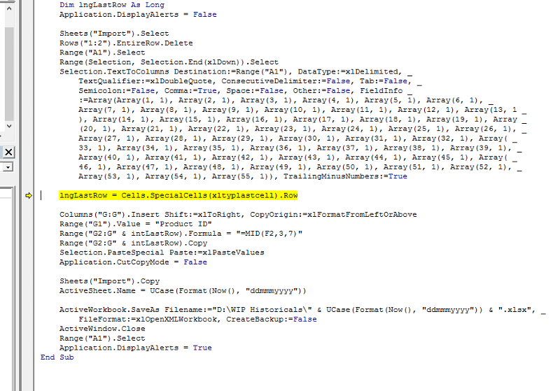
ASKER
Just for Your information ...
This is My home PC So i changed path.
Thanks
This is My home PC So i changed path.
Thanks
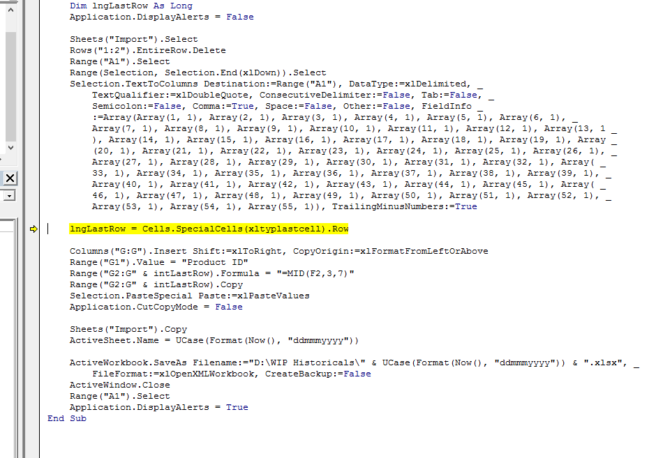
Yes, that's a typo. The line should be
My apologies.
lngLastRow = Cells.SpecialCells(xlCellTypeLastCell).RowMy apologies.
ASKER
Still There Is Error...See Attached WB. Will You Add Button In Sheet Import Which Execute Macro ...I Did But When I Run Macro It Disappeared ...Need Static Button.
Thanks
EE-Sample-TT-V-1.0.xlsm
Thanks
EE-Sample-TT-V-1.0.xlsm
ASKER CERTIFIED SOLUTION
membership
This solution is only available to members.
To access this solution, you must be a member of Experts Exchange.
ASKER
Yeah Its Working As Expected.May i Ask FollowUp?
Thanks
Thanks
Sure; open a new question unless it's very simple.
The change to 5) and 6) are accomplished by using a variable - lngLastRow - to determine the last row in the data and incorporate it into the formulas.
The change to 8) and 10) use this - UCase(Now(), "ddmmmyyyy") - to produce the date string for the sheet name and new workbook name.
The code - Application.DisplayAlerts - at the start and end of the macro allows the SaveAs function at the end to overwrite the file without any prompting.
Open in new window
Regards,
-Glenn