Excel 2016: auto-number column of merged cells.
Excel 2016/Win 10:
Hello,
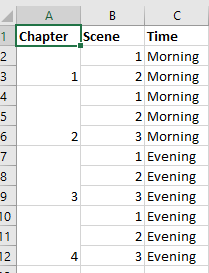
Please see the attached scrubbed spreadsheet (scene schedule for a novel). The first column (chapter) contains merged cells b/c chapters can contain multiple scenes.
Now, I need to combine chapters. So, what's originally:
Becomes:
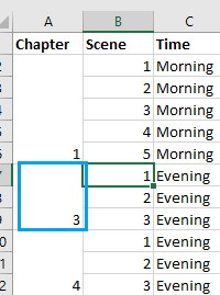
But I need to renumber Chapter 3 to Chapter 2, Chapter 4 to Chapter 3, etc. (No big deal for the sample, but the novel contains over 100 chapters).
I can't use ROW()-1 to autonumber, since the chapter cells encompass multiple rows. Accordingly, is there another way to auto-number these merged cells?
The attached sheet represents the layout before I combined Chapter 1 and Chapter 2.
Thanks,
Steve
Scene-Schedule---Scrubbed---for-EE.xlsx
Hello,
Please see the attached scrubbed spreadsheet (scene schedule for a novel). The first column (chapter) contains merged cells b/c chapters can contain multiple scenes.
Now, I need to combine chapters. So, what's originally:
Becomes:
But I need to renumber Chapter 3 to Chapter 2, Chapter 4 to Chapter 3, etc. (No big deal for the sample, but the novel contains over 100 chapters).
I can't use ROW()-1 to autonumber, since the chapter cells encompass multiple rows. Accordingly, is there another way to auto-number these merged cells?
The attached sheet represents the layout before I combined Chapter 1 and Chapter 2.
Thanks,
Steve
Scene-Schedule---Scrubbed---for-EE.xlsx
ASKER
@Rgonzo1971
Not quite.
1. Values are not correct.
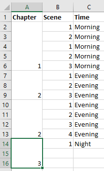
2. When I copied to the last row, it created a cell in col. A that merges alongside three cells in col. B. (Previously, there was no such merge).
3. The formula bar display the following for the two pasted cells.
a. Per Rows 10-13: the number 2.
b. Per Rows 14-16: =MAX(A$2:$A9)+1
Thanks.
Not quite.
1. Values are not correct.
2. When I copied to the last row, it created a cell in col. A that merges alongside three cells in col. B. (Previously, there was no such merge).
3. The formula bar display the following for the two pasted cells.
a. Per Rows 10-13: the number 2.
b. Per Rows 14-16: =MAX(A$2:$A9)+1
Thanks.
it works on your dummy
what are the formulas in the first and the second 2?
what are the formulas in the first and the second 2?
ASKER
=MAX(A2:$A$2)+1
2
Thanks.
2
Thanks.
only the first one (1) isn't a formula
Scene-Schedule---Scrubbed---for-EEv.xlsx
Scene-Schedule---Scrubbed---for-EEv.xlsx
ASKER
Understood. But that's what seemed to happen when I copied the original cell with the formula. Let me try again. Will get back to you in a few min. Thanks.
ASKER
Yeah, when I copy/paste, the number 2 absolutely appears in the formula bar.
And for the last copy, it converts the target cell into a merged cells.
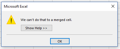
One thought: I had to type the formula manually. Because, when I copy/paste from this EE Thread (into the cell), it throws this error:
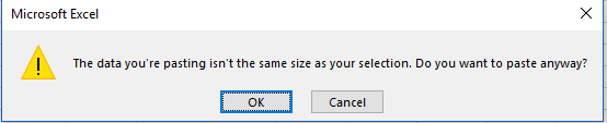
If I say I want to continue, I see:
--
Anyhow, I just downloaded your copy of my spreadsheet.
The formula I see above differs from what I saw in your original comment:
Which one is correct? Thanks.
And for the last copy, it converts the target cell into a merged cells.
One thought: I had to type the formula manually. Because, when I copy/paste from this EE Thread (into the cell), it throws this error:
If I say I want to continue, I see:
--
Anyhow, I just downloaded your copy of my spreadsheet.
=+MAX(A$2:$A2)+1The formula I see above differs from what I saw in your original comment:
=MAX(A2:$A$2)+1Which one is correct? Thanks.
both are equivalent for the purpose
you trying to copy and paste the formula you should fill down (Ctrl+D)
you trying to copy and paste the formula you should fill down (Ctrl+D)
This will work:
Step 2. Press F2, or click the Formula Bar, enter the formula: =MAX(A$1:A1)+1.
Step 3. Press CTRL+ENTER.
=MAX(A$1:A1)+1Step 2. Press F2, or click the Formula Bar, enter the formula: =MAX(A$1:A1)+1.
Step 3. Press CTRL+ENTER.
If you want VBA then try below:
Sub NumberCellsAndMergedCells()
    Dim Rng As Range
    Dim WorkRng As Range
    On Error Resume Next
    Set WorkRng = Range("A1:A16") ' Change your range here

    Set WorkRng = WorkRng.Columns(1)
    xIndex = 1
    Set Rng = WorkRng.Range("A1")
    Do While Not Intersect(Rng, WorkRng) Is Nothing
        Rng.Value = xIndex
        xIndex = xIndex + 1
        Set Rng = Rng.MergeArea.Offset(1)
    Loop
End Sub
Max formula will work only if your merged cells are identical. VBA works perfect with any merged cell size.
ASKER
OK, I followed steps 1-3 (In the file I downloaded from you it's A2:A12 but no matter). So far, so good. Now, the real test.
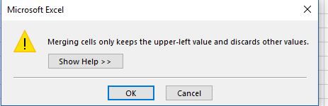
I want to merge the first two merged cells in Col. A. In effect, A2-A3 and A4-A6. I removed the value from the 2nd cell, and merge. Now, the "3" in rows 7-9 becomes "2", and the "4" in rows 10-12 becomes "3".
But when I try to do the merge, I saw
:
But wouldn't you know it, now that I'm trying to reproduce the error, I can't.
The above all looks good. However, I should mention this caveat: If I copy/paste a merged cell (e.g.) that has three rows in the other columns, it creates a new cell with four rows in the other columns. I suspect that behavior happens w/o your formula being involved, but wanted to let you know.
Thanks.
ASKER
@Shums -When you say:
>>Max formula will work only if your merged cells are identical. VBA works perfect with any merged cell size.
Please clarify "identical". Thanks.
>>Max formula will work only if your merged cells are identical. VBA works perfect with any merged cell size.
Please clarify "identical". Thanks.
Means the rows, in your case, some are 2 rows some are 3.
Try VBA then you will see the difference.
Try VBA then you will see the difference.
ASKER
@Shums-
What exactly does the MAX formula do? And, can I assume I need to save this spreadsheet as macro-enabled?
@All
Stepping out for a while. Will get back to you later. Thank you both!
What exactly does the MAX formula do? And, can I assume I need to save this spreadsheet as macro-enabled?
@All
Stepping out for a while. Will get back to you later. Thank you both!
Yes save your workbook with macro enabled.
ASKER
@Shums - I'm trying to create the macro, but the CREATE choice is grayed out...
Also: per line 5:
Set WorkRng = Range("A1:A16") ' Change your range here
Do I have to change the upper limit every time I add/remove a row? Or can I just type a large value? (e.g. 1000, as I know I'll never have that many scenes in the novel.)
Thanks.
Also: per line 5:
Set WorkRng = Range("A1:A16") ' Change your range here
Do I have to change the upper limit every time I add/remove a row? Or can I just type a large value? (e.g. 1000, as I know I'll never have that many scenes in the novel.)
Thanks.
Stephen,
Please find attached...Change your range as needed in module.
Auto-Number-in-Merged-Cell.xlsm
Please find attached...Change your range as needed in module.
Auto-Number-in-Merged-Cell.xlsm
ASKER
1. When I run it, it inserts the number 5 in cell A16. Funny thing: it's right-justified and all the other #s are centered.
2. How do I copy/paste this macro into my live spreadsheet?
Thanks.
2. How do I copy/paste this macro into my live spreadsheet?
Thanks.
Because in my example range is A1 to A16. Now you tell me your range and which column you wanted numbering?
ASKER
I realize why it calculated "5". Was wondering only per how the number was justified.
Please provide instructions/hints for pasting into live workbook. Thanks.
Please provide instructions/hints for pasting into live workbook. Thanks.
1. In your workbook Press Alt+F11 to activate VBE
2. Click your workbook name in the Project Window.
3. Choose Insert - Module to insert a VBA Module into the project
4. Paste the following code in the module
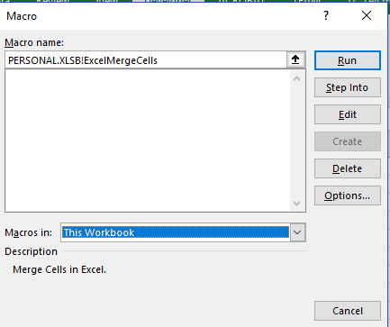
6. Go to Developer Menu, Click Macro
7. Click on NumberCellsAndMergedCells & press Run
Doesn't matter how long is your range, it will select last range until Column B, if your Scene has all the data.
Hope this helps.
2. Click your workbook name in the Project Window.
3. Choose Insert - Module to insert a VBA Module into the project
4. Paste the following code in the module
Sub NumberCellsAndMergedCells()
    Dim WS As Worksheet
    Dim LR As Long
    Dim Rng As Range
    Dim WorkRng As Range
    Set WS = ActiveSheet
    LR = WS.Range("B" & Rows.Count).End(xlUp).Row 'Change As Needed
    On Error Resume Next
    Set WorkRng = WS.Range("A2:A" & LR) ' Change your range here

    Set WorkRng = WorkRng.Columns(1)
    xIndex = 1
    Set Rng = WorkRng.Range("A1")
    Do While Not Intersect(Rng, WorkRng) Is Nothing
        Rng.Value = xIndex
        xIndex = xIndex + 1
        Set Rng = Rng.MergeArea.Offset(1)
    Loop
End Sub6. Go to Developer Menu, Click Macro
7. Click on NumberCellsAndMergedCells & press Run
Doesn't matter how long is your range, it will select last range until Column B, if your Scene has all the data.
Hope this helps.
ASKER
Nice! I tried it on my test workbook with promising results. Will soon try it on live workbook.
Just curious: Do your comments about changing as needed (line 7) and changing range (line 9) no longer apply?
Thank you!
Just curious: Do your comments about changing as needed (line 7) and changing range (line 9) no longer apply?
Thank you!
Line 7 is is taking the last line of the column which has complete data. In my example I used Column B, so you can change whichever column has data until last row.
Line 9 is the working range where you want the auto numbering, I selected from A2 till last row of A, so you can change where you want numbering to be.
Hope this helps.
Line 9 is the working range where you want the auto numbering, I selected from A2 till last row of A, so you can change where you want numbering to be.
Hope this helps.
Kindly Note, this VBA auto number Merged or normal cells.
ASKER
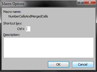
Got it. Final question: is there a way to assign a hotkey to this macro? Thanks.
Follow below steps:
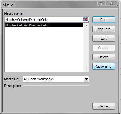 Then Click Option and assign any key:
Then Click Option and assign any key:
ASKER
Ok, I assigned CTRL-L, but when I pressed that key combination, it invoked the Create Table dialog. How can i find a keystroke sequence that's not used? Thanks.
Be careful assigning your own Key for macro, please check the list of shortcuts already assigned my Microsoft here Excel keyboard shortcuts and function keys for Windows
Pressing SHIFT + CTRL + S to run your own macro is reasonable (this key doesn't do anything else in Excel)
Pressing SHIFT + CTRL + S to run your own macro is reasonable (this key doesn't do anything else in Excel)
ASKER
My bad. I missed the "shift" on the screen where I assigned the keystroke. Your suggestion worked.
No need for you to respond further. I'll work with the macro as I revise the live scene schedule. Once I'm satisfied it works for me, I'll close the question.
Thanks again for your patient help.
Steve
No need for you to respond further. I'll work with the macro as I revise the live scene schedule. Once I'm satisfied it works for me, I'll close the question.
Thanks again for your patient help.
Steve
You're welcome Sir Steve! Glad I was able to help.
Just last request, please add VBA in your topic as you gonna use VBA for your solution.
ASKER
How can I edit the question title/topics/? It may be too late b/c comments have been posted...
ASKER
Shums,
Seems like I accidentally ran the macro on another spreadsheet, which had dates in the first column. It changed all the dates to what I guess is the equivalent of the sequence 1, 2, 3. e.g. 1/1/1900, 1/2/1900. Fortunately ,I had a backup of this sheet, so no harm done. However,
Can the macro be modified so that it will run ONLY on the spreadsheet with a given filename? I often have multiple workbooks open, so it's possible I could make the same mistake again.
Thanks,
Steve
Steve,
I can specify Worksheet name, but it wont work on several workbooks as sheet name may differ, that's why in my code I specified Active Sheet.
Whichever Workbook you gonna open, paste this code in module and select the sheet where you need Auto Numbering and run this macro.
I can specify Worksheet name, but it wont work on several workbooks as sheet name may differ, that's why in my code I specified Active Sheet.
Whichever Workbook you gonna open, paste this code in module and select the sheet where you need Auto Numbering and run this macro.
ASKER
Thanks. Worksheet name would be useful. I can always change it to match the name of my workbook. :)
ASKER CERTIFIED SOLUTION
membership
This solution is only available to members.
To access this solution, you must be a member of Experts Exchange.
ASKER
Thank you. Will try later today.
ASKER
Results:
Ran on the sheet for which it was intended: Looks good.
Ran on another sheet in same workbook: apparently does not run, which is as intended. This sheet has text in the first column.
Ran on a sheet in another workbook: Runtime error '9' - subscript out of range This sheet has dates in the first column.
I'd rather it run w/o the error in the last use case.
Thanks.
Sir,
That's why I had ActiveSheet as Sheet Name. If you forgets to change Sheet Name or if you select wrong range, you will get such error. I also told you, the VBA I provided was for your sample file, if you gonna use for another workbook, then please check the range wherever I wrote 'Please change the range as required'
There is nothing wrong with the code, if you gonna miss one minor thing, you gonna end up error.
Sorry about problems caused.
ASKER
Understood. But, shouldn't the macro not run at all when I run on a sheet whose name is not the same as the one designated? Thanks.
No Sir It won't run
As I mentioned in my code
As I mentioned in my code
On Error Resume NextASKER
Well, if it threw the error, sounds like to me that it ran? Or, am I missing something....Thanks.
Sir,
I tested many times, and it worked perfectly.
I tested many times, and it worked perfectly.
Sir,
Refer to your subject, you asked for Auto-numbering Merged cell, which I already provided you, even to teach you how to insert VBA code, how to assign shortcut keys to any macro, provided sample file which you can refer.
I request you to please close this question and raise another one for further proceedings.
SOLUTION
membership
This solution is only available to members.
To access this solution, you must be a member of Experts Exchange.
ASKER
Thank you again, Shums.
Rgonzo - Apologies I could not give you points, but b/c of the limitations of your solution, I could not accept as a viable method. Feel free to disagree, in which case I will contact the mods to see if you can receive credit.
Thanks.
Rgonzo - Apologies I could not give you points, but b/c of the limitations of your solution, I could not accept as a viable method. Feel free to disagree, in which case I will contact the mods to see if you can receive credit.
Thanks.
pls try in cell A4 and fill down
Open in new window
Regards