Macro Lookup

Sample formulas included in attached sheet.  Copy down for additional rows as needed.

~bp
EE28997192.xlsx

And actually I think I approached that too simply.  I think you really wanted to search the whole column range looking for the value, not just the single row.  This approach should handle that.

~bp
EE28997192.xlsx

You can use below code as well:

Sub UpdateFormula()
Dim Ws As Worksheet
Dim LR As Long
Set Ws = ActiveSheet
LR = Ws.Range("A" & Rows.Count).End(xlUp).Row
Ws.Range("C2:C" & LR).FormulaR1C1 = _
        "=IFERROR(IF(OR(VLOOKUP(RC2,C7,1,0),VLOOKUP(RC2,C8,1,0))=RC2,RC9,""""),""PC not Available"")"
Ws.Range("D2:D" & LR).FormulaR1C1 = _
        "=IFERROR(IF(OR(VLOOKUP(RC2,C11,1,0),VLOOKUP(RC2,C12,1,0))=RC2,RC13,""""),""PC not Available"")"
Ws.Range("E2:E" & LR).FormulaR1C1 = _
        "=IFERROR(IF(OR(VLOOKUP(RC2,C15,1,0),VLOOKUP(RC2,C16,1,0))=RC2,RC17,""""),""PC not Available"")"
End Sub

Select allOpen in new window

Bill as per your formula

 =INDEX($I$2:$I$19,MATCH(1,($B2>=$G$2:$G$19)*($B2<=$H$2:$H$19),0)) 

Select allOpen in new window

you are checking the product code which are greater than or equals to the product code, as per author, he needs exact match. That's why your formula showing the value of few Product Codes.

Secondly, he wanted VBA to update automatically 15000 rows, if he gonna use Index-Match function, its gonna be very slow.

You are very senior and I know you can get best VBA code to do this lookup.

Hi Shums,
your VBA is not returning any values.
PC not available on all.

Shums,

In my formula, I am actually doing a MATCH where the result of "is this value between two values in the lookup table" is true.  It looks a little odd because the way I chose to do that was with MATCH, looking for the value 1, and then computing an array product of the two conditions, is the column B value >= to the column G value (this will return 0 for false, 1 for true) multiplied by is the column B value >= to the column H value (this will return 0 for false, 1 for true).  So we will only get a value 1 when both of these are true, which is what we want.  When that is true we get the row index and use that in the INDEX function to get the value from column I.

~bp

W.E.B

Do you have the full set of data that I can test performance with please?

~bp

Hi Bill,
I'm testing your formula,
when I hit the enter on any of the cells, it changes to #N/A (Even though a value is found).
Example Cells --- c2,c3,c4 ....

If you are updating the formulas I created, they are array formulas, so you have to press ctl-shift-enter rather than enter.

Notice in the sheet I provided the formulas have curly braces {} around them, that indicates an array formula.

~bp

Try below code:

Sub UpdateFormula()
Dim Ws As Worksheet
Dim LR As Long
Set Ws = ActiveSheet
LR = Ws.Range("A" & Rows.Count).End(xlUp).Row
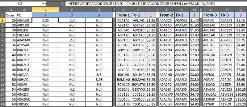
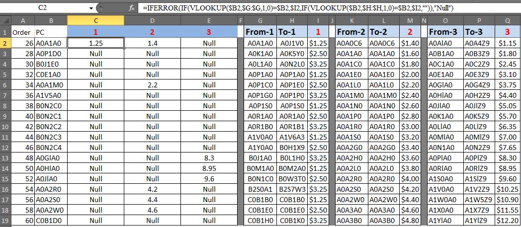
Ws.Range("C2:C" & LR).FormulaR1C1 = "=IFERROR(IF(VLOOKUP(RC2,C7,1,0)=RC2,RC9,IF(VLOOKUP(RC2,C8,1,0)=RC2,RC9,"""")),""Null"")"
Ws.Range("D2:D" & LR).FormulaR1C1 = "=IFERROR(IF(VLOOKUP(RC2,C11,1,0)=RC2,RC13,IF(VLOOKUP(RC2,C12,1,0)=RC2,RC13,"""")),""Null"")"
Ws.Range("E2:E" & LR).FormulaR1C1 = "=IFERROR(IF(VLOOKUP(RC2,C15,1,0)=RC2,RC17,IF(VLOOKUP(RC2,C16,1,0)=RC2,RC17,"""")),""Null"")"
End Sub

Select allOpen in new window

Bill,
I'm testing your formula now, is there any way to avoid the ctl-shift-enter?

Shums,
I'm still not getting the values.
getting Null

Wass,

Please see below capture, it is showing the matching values.

In Column G, there is only one matching Values of Column B

Try above code in your original workbook and check

With my formula, since they use array formulas, they must be entered with ctl-shift-enter.  But that is only when they are first entered, after that you shouldn't need to touch them, right?  They can be copied with normal copy and paste method.

Also, I would strongly suggest you use named ranges for the various cell ranges, that way the formulas would not have to change if additional rows were added down the road, just the defined named range would be adjusted in one place.  Much easier than having to update all the formulas.

~bp

Hi Shums,
I just tried on a new sheet
C2, Null
D2 Null

PC      1      2      3
A0A1B0      Null      Null      Null
A0P1D0      Null      Null      Null
B0J1E0      Null      Null      Null
C0E1A0      Null      Null      Null
A0A1M0      Null      2.2      Null
A1V5A0      Null      Null      Null
B0N2C0      Null      Null      Null
B0N2C1      Null      Null      Null
B0N2C2      Null      Null      Null
B0N2C3      Null      Null      Null
B0N2C4      Null      Null      Null
A0GlA0      Null      Null      8.3
A0HlA0      Null      Null      8.95
A0JlA0      Null      Null      9.6
A0A2R0      Null      4.2      Null
A0A2S0      Null      4.4      Null
A0A2W0      Null      4.6      Null
C0B1D0      Null      Null      Null

One other thought, does this absolutely have to be Excel.  It might work out better in Access, where you could have a table column B, and then one table each for the 1, 2, 3 lookup data.  Then using the power of a JOIN in Access it would be pretty easy to pull together the additional columns you want for each line.  Just a thought...

~bp

Please send screen shot of result columns with all other matching columns.

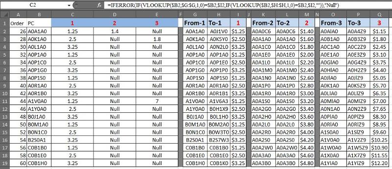
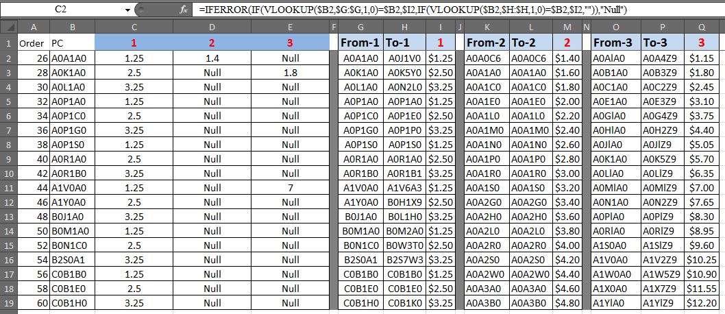
I just copy pasted the content of column G to column B and see the formula result:

Please see attached.
I'm using Excel 2007 (case it makes any difference)
test.xlsx

No Excel version doesn't make any difference. Code and formula are right, its just the sample codes what you are picking have no match.

Manually you can check copying few PC and try to find, it will not show any result.

Shums,

Your approach has a problem in that it is using VLOOPUP and the exact match option, so you are only getting data when the value in column B is an exact match to the data table.  However, in B3 we have A0P1D0, which falls in the "1" range on row 6 of A0P1C0 to A0P1E0.  But your formula does not find that.

Also, your VLOOKUP approach will only work if all the data in columns G, H, K, L, O, P are sorted.  I wasn't sure if that assumption could be made even though it seems to be true in the example data.

~bp

That's nice explanation. Here come's seniority. :)

My bad, I misread it.

Thanks for correcting me.

W.E.B.

I don't understand of looking in the full range of Column B, as Vlookup is looking each row of Column B in the column G, H, K, L, O & P.

Here is the attached file in 3 different ways in 3 different sheets. Only the first Vlookup works fine.
First way:

Sub UpdateFormula1()
Dim ws As Worksheet
Dim LR As Long
Set ws = Sheets("Sheet2")
LR = ws.Range("A" & Rows.Count).End(xlUp).Row
ws.Range("C2:C" & LR).FormulaR1C1 = "=IFERROR(IF(VLOOKUP(RC2,C7,1,0)=RC2,RC9,IF(VLOOKUP(RC2,C8,1,0)=RC2,RC9,"""")),""No Match"")"
ws.Range("D2:D" & LR).FormulaR1C1 = "=IFERROR(IF(VLOOKUP(RC2,C11,1,0)=RC2,RC13,IF(VLOOKUP(RC2,C12,1,0)=RC2,RC13,"""")),""No Match"")"
ws.Range("E2:E" & LR).FormulaR1C1 = "=IFERROR(IF(VLOOKUP(RC2,C15,1,0)=RC2,RC17,IF(VLOOKUP(RC2,C16,1,0)=RC2,RC17,"""")),""No Match"")"
ws.Columns("C:E").EntireColumn.AutoFit
End Sub

Select allOpen in new window

Second way:

Sub FindValuesAndUpdateCells()

Dim lastRow As Long
Dim tempVal As String

    lastRow = Sheets("Sheet1").Range("A" & Rows.Count).End(xlUp).Row

    For sRow = 2 To lastRow
        tempVal = Sheets("Sheet1").Cells(sRow, "B").Text

        For tRow = 2 To lastRow
            If Sheets("Sheet1").Cells(tRow, "G") = tempVal Or Sheets("Sheet1").Cells(sRow, "H") = tempVal Then
                Sheets("Sheet1").Cells(tRow, "C") = Sheets("Sheet1").Cells(sRow, "I")
            End If
            If Sheets("Sheet1").Cells(tRow, "K") = tempVal Or Sheets("Sheet1").Cells(sRow, "L") = tempVal Then
                Sheets("Sheet1").Cells(tRow, "D") = Sheets("Sheet1").Cells(sRow, "M")
            End If
            If Sheets("Sheet1").Cells(tRow, "O") = tempVal Or Sheets("Sheet1").Cells(sRow, "P") = tempVal Then
                Sheets("Sheet1").Cells(tRow, "E") = Sheets("Sheet1").Cells(sRow, "Q")
            End If
        Next tRow
    Next sRow

Dim match As Boolean
'now if no match was found, then put NO MATCH in cell
    For lRow = 2 To lastRow
        match = False
        tempVal = Sheets("Sheet1").Cells(lRow, "B").Text

        For sRow = 2 To lastRow
            If Sheets("Sheet1").Cells(sRow, "G") = tempVal Or Sheets("Sheet1").Cells(sRow, "H") = tempVal Then
                match = True
            End If
            If Sheets("Sheet1").Cells(sRow, "K") = tempVal Or Sheets("Sheet1").Cells(sRow, "L") = tempVal Then
                match = True
            End If
            If Sheets("Sheet1").Cells(sRow, "O") = tempVal Or Sheets("Sheet1").Cells(sRow, "P") = tempVal Then
                match = True
            End If
        Next sRow

        If match = False Then
            Sheets("Sheet1").Cells(lRow, "C") = "NO MATCH"
            Sheets("Sheet1").Cells(lRow, "D") = "NO MATCH"
            Sheets("Sheet1").Cells(lRow, "E") = "NO MATCH"
        End If
    Next lRow
Sheets("Sheet1").Columns("C:E").EntireColumn.AutoFit
End Sub

Select allOpen in new window

Third way:

Sub UpdateFormula2()
Dim ws As Worksheet
Dim LR As Long
Set ws = Sheets("Sheet3")
LR = ws.Range("A" & Rows.Count).End(xlUp).Row
ws.Range("C2:C" & LR).FormulaR1C1 = "=IFERROR(IF(VLOOKUP(RC7,C2,1,0)=RC7,RC9,IF(VLOOKUP(RC8,C2,1,0)=RC8,RC9,"""")),""No Match"")"
ws.Range("D2:D" & LR).FormulaR1C1 = "=IFERROR(IF(VLOOKUP(RC11,C2,1,0)=RC11,RC13,IF(VLOOKUP(RC12,C2,1,0)=RC12,RC13,"""")),""No Match"")"
ws.Range("E2:E" & LR).FormulaR1C1 = "=IFERROR(IF(VLOOKUP(RC15,C2,1,0)=RC15,RC17,IF(VLOOKUP(RC16,C2,1,0)=RC16,RC17,"""")),""No Match"")"
ws.Columns("C:E").EntireColumn.AutoFit
End Sub

Select allOpen in new window

Please advice.
Sample_Vlookup_V2.xlsm

W.E.B.

Where are you with the earlier solution I proposed that seemed to work?  Is there something additional you need from it?

~bp

Hi Shums,
it seems, your code only works if their is an exact match,
it's not looking up if the value falls between ...
Example
Cell B2 = A0A1B0     (Falls Between A0A1A0      A0J1V0)        It should have returned the value   1.25
Cell B3 = A0P1D0     (Falls between A0P1C0      A0P1E0)       It should have returned the value   2.50

If I put exact Matches, your code works

Hi Bill,
I'm still trying to figure out how to avoid the ctrl-shift-enter.
those postal codes will change weekly,

Appreciate the help.

Thanks W.E.B. I can change that.

OK try below and I am being honest, I am using Bill's formula in below VBA:

Sub UpdateFormula()
Dim ws As Worksheet
Dim LR As Long
With Application
    .ScreenUpdating = False
    .DisplayStatusBar = True
    .StatusBar = "!!! Please Be Patient...Updating Records !!!"
    .EnableEvents = False
    .Calculation = xlManual
End With

Set ws = ActiveSheet
LR = ws.Range("A" & Rows.Count).End(xlUp).Row
ws.Range("C2").FormulaArray = _
        "=IFERROR(INDEX(Result1,MATCH(1,($B2>=From_1)*($B2<=To_1),0)),""No Match"")"
ws.Range("C2:C" & LR).FillDown
ws.Range("D2").FormulaArray = _
        "=IFERROR(INDEX(Result2,MATCH(1,($B2>=From_2)*($B2<=To_2),0)),""No Match"")"
ws.Range("D2:D" & LR).FillDown
ws.Range("E2").FormulaArray = _
        "=IFERROR(INDEX(Result3,MATCH(1,($B2>=From_3)*($B2<=To_3),0)),""No Match"")"
ws.Range("E2:E" & LR).FillDown

With Application
    .ScreenUpdating = True
    .DisplayStatusBar = True
    .StatusBar = False
    .EnableEvents = True
    .Calculation = xlAutomatic
End With
ws.Range("C2:E" & LR).Value = ws.Range("C2:E" & LR).Value
ws.Columns("C:E").AutoFit
ws.Range("B2").Select
End Sub

Select allOpen in new window

Bill if you have better VBA version, you can post.

Shums,
all values are being entered in Column C

Bill,
I just saw your code,
testing now.

Oops, Please find attached...
Sample_Vlookup_V3.xlsm

Guys,
Thank you very VERY much for your help.
Much appreciated.

@ W.E.B. thanks for considering me.
@ Bill, hats off to you sir