Excel VLookup Function Help
Hi,
I need help creating a VLookup function in Excel 2016 for Mac. I have struggled with this problem for years, and I am finally asking for help! ;-)
I need to find the ID for each analytical technique from Column E which will populate Column C.
Here is the formula I created in the attached file:
=B3=VLOOKUP(C3,E:H,0,TRUE)
Please tell me what I have done wrong.
VLookupTags-4-28-17.csv
Edward Pamias
take off the =b3 and can you send an XLSX file instead please.
And by the looks of your file you have nothing in column C to lookup.
You also need to replace 0 to which column you are pulling, try below, change 2 as per your need:
=VLOOKUP(C3,E:H,2,TRUE)ASKER
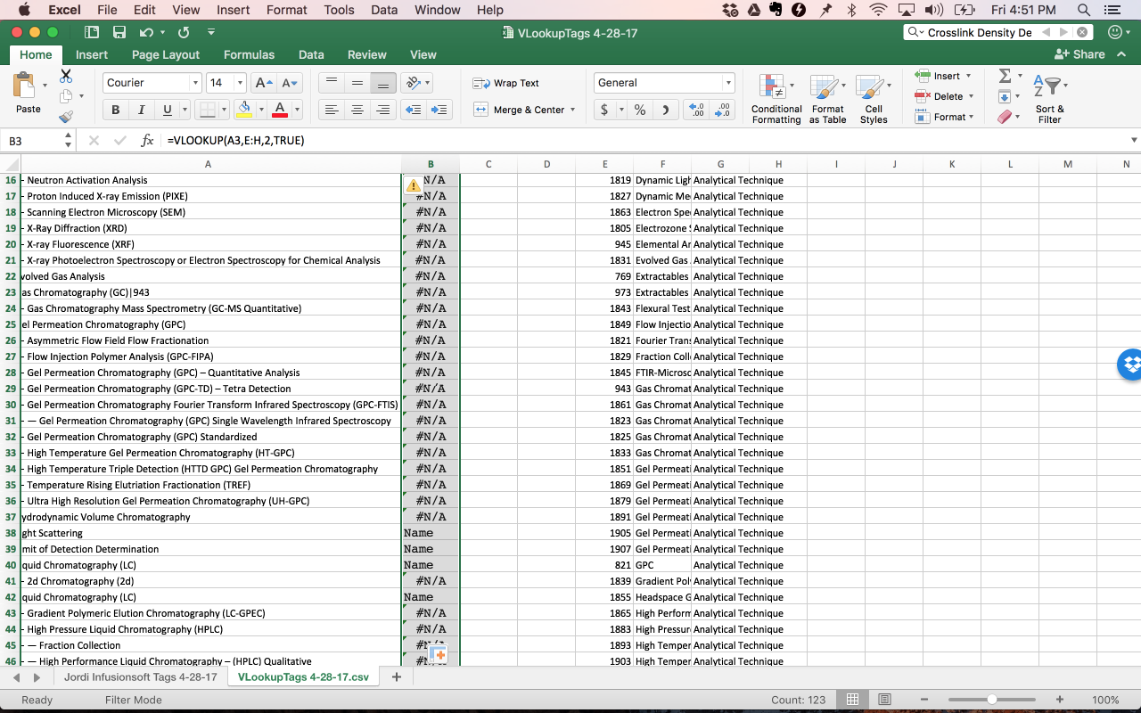
Thanks @Shums. That did not work. Here is the result.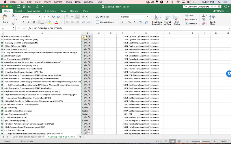
In Column A you have Techniques and you are looking up IDs, it wont work.
What exactly you are looking and what is your expected result. please upload a sample workbook.
What exactly you are looking and what is your expected result. please upload a sample workbook.
Try below Array Formula (Confirmed with Ctrl+Shift+Enter):
=IFERROR(INDEX(E$2:E$112,MATCH(TRUE,ISNUMBER(SEARCH(F$2:F$112,A2)),0)),"")
@ Author,
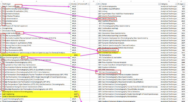
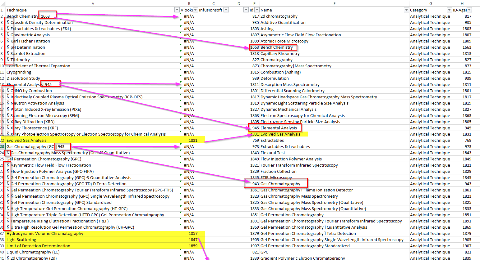
I think your problem is that you are trying to return the 1st column E, by matching on the second column F, and want the match to be based on Column A
The vlookup function requires the matching column to be the 1st column in your set fo columns.
To do this you need to re-arrange your columns so that Column E and ColumnF are switched and changed your vLookup formula to:
Or as I did you can put an = and replicate the ID column at the end in Column H
However, by matching on Column A you are not going to get many matches because the data there is a scrape from somewhere and is full of extra characters and such (see screenshot ofdf my test).
PS don;t use CSVs, they DO NOT keep formulas, and they DO NOT give all the pages of the workbook, so we only get a limited view. Send an XLSX, or XLS instead.
I think your problem is that you are trying to return the 1st column E, by matching on the second column F, and want the match to be based on Column A
The vlookup function requires the matching column to be the 1st column in your set fo columns.
To do this you need to re-arrange your columns so that Column E and ColumnF are switched and changed your vLookup formula to:
=VLOOKUP(C3,E:H,2,TRUE)Or as I did you can put an = and replicate the ID column at the end in Column H
However, by matching on Column A you are not going to get many matches because the data there is a scrape from somewhere and is full of extra characters and such (see screenshot ofdf my test).
PS don;t use CSVs, they DO NOT keep formulas, and they DO NOT give all the pages of the workbook, so we only get a limited view. Send an XLSX, or XLS instead.
I sent him the file fixed. I removed all the special characters earlier and created the vlookup.
ASKER CERTIFIED SOLUTION
membership
This solution is only available to members.
To access this solution, you must be a member of Experts Exchange.
ASKER
This is great. Can you please explain to me how this works?
The LOOKUP function is included for compatibility in Excel because Lotus 123 had it, but most people correctly ignore it in favor of VLOOKUP, HLOOKUP or INDEX & MATCH. Where LOOKUP comes into its own is when you take advantage of some of its more esoteric properties.
1. Although Microsoft documentation suggests that the second parameter in LOOKUP must be sorted in ascending order, that does not need to be the case. In actual fact, close to 100% of my uses of LOOKUP aren't sorted.
2. LOOKUP works like an array-entered function, but does need to be array-entered
3. When LOOKUP cannot find an exact match in a properly sorted search array, it returns as a match the last value of the same variable type as the first parameter. In other words, it ignores error values. By variable type, I mean text, numeric, or error value.
4. If LOOKUP has only two parameters, it returns the last matching value as described in #3. But if there are three parameters, LOOKUP returns a value from the array in the third parameter in the same position as the match in the second parameter.
5. LOOKUP returns an error value if there are no values in the second parameter of the same type as the first parameter.
In my suggested formula:
SEARCH(F$2:F$112,A2) examines cell A2 for the various substrings found in F2:F112. It returns an array of values consisting of the character position number where a match was found in cell A2 and error values.
1/SEARCH(F$2:F$112,A2) returns an array of either error values or values somewhere between 0 and 1
LOOKUP wants to find 2, which will never be found in the array returned by 1/SEARCH(...). So it instead returns a match for the very last numeric value found in that array (i.e. the same variable type as the 2 in the first parameter).
Since there are three parameters, LOOKUP returns a value from E2:E112 that corresponds to the match from F2:F112.
In your particular problem, there may be more than one lab procedure substring in column F that match the text in cell A2. You want the match to be as greedy as possible to match the longest such substring. With alphabetical order, the greediest matches always occur after less greedy matches, so you need a LOOKUP type of solution.
Note that you can still seize defeat from the jaws of victory if some of your procedures have Frankenstein type names. For example "Fuel analysis: heat of combustion & heavy metals" would be incorrectly ignored in favor of "Heavy metals" because it sorts later in alphabetical order. I didn't recall seeing any examples of these pitfalls, but can imagine the possibility. The cure is to make sure the shorter string appears before the longer one in the list of lab procedures.
Nice work Brad,
Please have a look, as you compared our solutions, there were 32 errors I found in your formula and 45 errors in mine.
It will always be difficult to find partial text in a string to get 100 % accurate result, as same partial text may appear in another sub strings.
Brad_VLookupTags-4-28-17_2.xlsx
Please have a look, as you compared our solutions, there were 32 errors I found in your formula and 45 errors in mine.
It will always be difficult to find partial text in a string to get 100 % accurate result, as same partial text may appear in another sub strings.
Brad_VLookupTags-4-28-17_2.xlsx
ASKER
Thank you so much for this explanation!
In my work, I often have to do similar types of data matching.
I was hoping I would be able to get a formula I could use somewhat universally, but it sounds like each V/LOOKUP formula has to be tailored quite specifically to the data.
Is there another way to structure the data that would lend itself to a formula that required less customization (and therefore less knowledge of Excel formulas)?
Thanks again to everyone who responded!
Josh
If you sort your lookup column by text length, that should do the needful. If you sort the lab procedures with the longest name first, then use Shums' INDEX & MATCH. If you sort with the shortest name first, then use the LOOKUP formula.