Excel DropDown menu - Based on cell value without a dropdown menu
Hi,
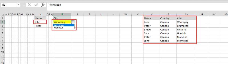
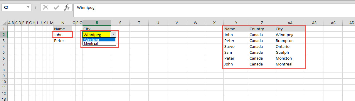
I would like to have a dynamic DropDown menu in cell "R2" that would adjust based on the value in "N2".
The cell in N2 will not have a DropDown menu.
The data reference will be in Column Y to AA.
So if i type "John" in cell N2, the DropDown menu from R2 will have the value ("Winnipeg" and "Montreal").
If the value in N2 does not exist in column Y, the DropDown items would be empty.
Is that possible? Is so, how can i do it?
Thank you for your help
Ex:
 DropDown-sample.xlsx
SOLUTION
membership
This solution is only available to members.
To access this solution, you must be a member of Experts Exchange.
I guess you need this
added a couple named ranges to make it simple to understand...
see sample
29063165.xlsx
=OFFSET($Y$2, MATCH(N2,NAMES,0)-1, 2, COUNTIF(NAMES,N2), 1)added a couple named ranges to make it simple to understand...
see sample
29063165.xlsx
ASKER
Hi HainKurt
It looks like this forlula doesn't really work. I cant really add other formula to make it work in the sheet.
=OFFSET($Y$2, MATCH(N2,NAMES,0)-1, 2, COUNTIF(NAMES,N2), 1)
Hi Subodh Tiwari (Neeraj)
I like this option. Let me test it a little more. Will be back soon.
It looks like this forlula doesn't really work. I cant really add other formula to make it work in the sheet.
=OFFSET($Y$2, MATCH(N2,NAMES,0)-1, 2, COUNTIF(NAMES,N2), 1)
Hi Subodh Tiwari (Neeraj)
I like this option. Let me test it a little more. Will be back soon.
Hi
I would arrange my dropdown sources in a different manner, using single column tables, with a table Name the same as the header .
Then the Validation is simply
=(INDIRECT(N2) etc.
If you have lots of tables to create for your source data, I have a simple macro as part of the tutorial on this method at
http://www.contextures.com/exceldatavaldependindextablesindirect.html
29063165-RJG.xlsx
ASKER
Hi rogergovier
That would require to change to transpose the table and at this moment, i can't.
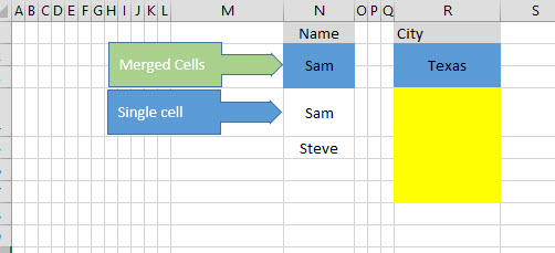
Subodh Tiwari (Neeraj), I'm having an problem when the row from column "N" and "R" are merged.
Ex:
N5 and N6 are merged together and also R5 and R6. How can i make the dropdown menu work?.
One thing is for sure, if rows from column N are merged, column R will also be merged with the same rows.
Thanks
That would require to change to transpose the table and at this moment, i can't.
Subodh Tiwari (Neeraj), I'm having an problem when the row from column "N" and "R" are merged.
Ex:
N5 and N6 are merged together and also R5 and R6. How can i make the dropdown menu work?.
One thing is for sure, if rows from column N are merged, column R will also be merged with the same rows.
Thanks
@Wilder1626
firstly, apologies for the superfluous ( in my formula - fat finger!!
It should read
=INDIRECT(N2)
Secondly, the data for the validation lists does not have to be contained on the same sheet, so I cannot see why you cannot transpose your data.
firstly, apologies for the superfluous ( in my formula - fat finger!!
It should read
=INDIRECT(N2)
Secondly, the data for the validation lists does not have to be contained on the same sheet, so I cannot see why you cannot transpose your data.
ASKER
@rogergovier
I understand what you are saying and it could be transposed but i didn't want to go that way cause that list also do other task, and i must keep it in the same format. I also don't want to create a duplication of that list just because i have to transpose it.
I understand what you are saying and it could be transposed but i didn't want to go that way cause that list also do other task, and i must keep it in the same format. I also don't want to create a duplication of that list just because i have to transpose it.
@Wilder1626
Hi
Fine, I understand.
But I see that you have a hidden sheet called dbase, which looks like it holds the data for your validation.
If you can accept a VBA solution, then the attached will work.
Basically there is event code on Master for both a Selection Change or a Change event.
These trigger a copy of the Name to cell G2 on hidden sheet dbase, and then invoke a macro called FilterData
This Macro, does an Advanced Filter to extract a list of the cities belonging to that person, and places then in G4 downward on sheet dbase
The macro then also creates a Named range for the depth of this data called Cities, which is what is then used in column R of sheets Master.
I hope that this helps
Sub FilterData()
    Dim wsS As Worksheet
    Dim lr As Long, lr2 As Long
    Dim myRange As Range

    Application.ScreenUpdating = False
    Set wsS = Sheets("Dbase")
    wsS.Activate
    With wsS
        lr = wsS.Cells(Rows.Count, 1).End(xlUp).Row
        wsS.Range("A1:C" & lr).AdvancedFilter Action:=xlFilterCopy, CriteriaRange:=wsS.Range( _
            "G1:G2"), CopyToRange:=wsS.Range("G3"), Unique:=False
        lr2 = wsS.Cells(Rows.Count, 7).End(xlUp).Row
        lr2 = Application.Max(4, lr2)
        Set myRange = Range(Cells(4, 7), Cells(lr2, 7))
        ActiveWorkbook.Names.Add Name:="Cities", RefersTo:=myRange
    End With
    Sheets("Master").Activate
    Application.ScreenUpdating = True
End SubASKER
@rogergovier
That looks very interesting. Let me test this. I will get back to you.
That looks very interesting. Let me test this. I will get back to you.
Hi,
Check the attached solution using indirect and helper columns beside the data source.
I have used same sheet @HainKurt posted.
29063165.xlsx
Check the attached solution using indirect and helper columns beside the data source.
I have used same sheet @HainKurt posted.
29063165.xlsx
ASKER
I've done multiple test and so far, it works as long cells are not merged. I also like the vba option.
Right now, this is a problem for me cause i could have merged cells also.
Ex:
N5 and N6 are merged together and also R5 and R6 together. How can i make the dropdown menu to work?.
One thing is for sure, if rows from column N are merged, column R will also be merged with the same rows.
Right now, this is a problem for me cause i could have merged cells also.
Ex:
N5 and N6 are merged together and also R5 and R6 together. How can i make the dropdown menu to work?.
One thing is for sure, if rows from column N are merged, column R will also be merged with the same rows.
SOLUTION
membership
This solution is only available to members.
To access this solution, you must be a member of Experts Exchange.
I thought I solved this before :)
the data should be sorted for this to work
have a look at this
29063165.xlsx
=OFFSET($Y$2, MATCH(N2,NAMES,0)-1, 2, COUNTIF(NAMES,N2), 1)the data should be sorted for this to work
Name	Country	City
John	Canada	Winnipeg
John	Canada	Montreal
Peter	Canada	Brampton
Peter	Canada	Moncton
Sam	Canada	Guelph
Steve Canada Ontariohave a look at this
29063165.xlsx
ASKER
@ HainKurt
The problem is that the data may not be sorted. So it would not work.
@ rogergovier, i agree with you that merged cell is really not the best and should be avoid at all time. But unfortunately, the file i need to work with as merged cells. Let me try it and will get back to you.
The problem is that the data may not be sorted. So it would not work.
@ rogergovier, i agree with you that merged cell is really not the best and should be avoid at all time. But unfortunately, the file i need to work with as merged cells. Let me try it and will get back to you.
you can just sort it, which I did...
just select those 3 columns and click sort...
is there any reason not to sort it, and go with vba solution instead?
just select those 3 columns and click sort...
is there any reason not to sort it, and go with vba solution instead?
ASKER
@ HainKurt
That file is being used and updated by multiple person. If they forgot to sort the sheet, it will cause other problems where they will be missing multiple options.
To reduce the risk, i would like to prevent to have to sort it to make it work. Unfortunately, i have to think about the pros and cons. In other circumstances, it would of been a good solution.
ok what about this
what I do here is, if you click/select a cell in column R (row<>1), then that code finds cities and creates dynamic validation based on value in N column...
29063165.xlsm
Private Sub Worksheet_SelectionChange(ByVal Target As Range)
    If Target.Row = 1 Or Target.Column <> 18 Or Target.Cells.Count > 1 Then Exit Sub

    Dim list As String
    Dim n As String
    n = Range("N" & Target.Row).Value
    For i = 2 To Range("NAMES").Rows.Count + 1
      If Range("Y" & i) = n Then list = IIf(list = "", Range("AA" & i).Value, list & ", " & Range("AA" & i).Value)
    Next

    With Selection.Validation
        .Delete
        .Add Type:=xlValidateList, AlertStyle:=xlValidAlertStop, Operator:=xlBetween, Formula1:=list
        .IgnoreBlank = True
        .InCellDropdown = True
        .InputTitle = ""
        .ErrorTitle = ""
        .InputMessage = ""
        .ErrorMessage = ""
        .ShowInput = True
        .ShowError = True
    End With

End Subwhat I do here is, if you click/select a cell in column R (row<>1), then that code finds cities and creates dynamic validation based on value in N column...
29063165.xlsm
ASKER
@HainKurt
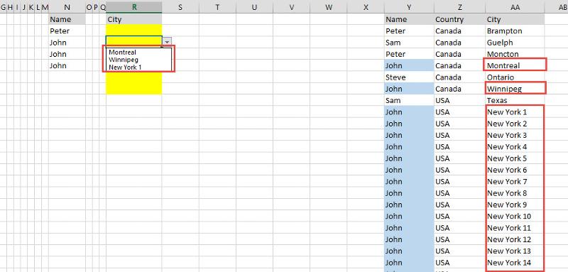
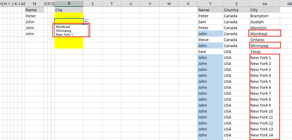
I just tried and if i add more name and cites, the drop down menu don't really adjust:
I just tried and if i add more name and cites, the drop down menu don't really adjust:
I just tried and if i add more name and cites, the drop down menu don't really adjust:
because I used named ranges...
if it is dynamic, we can use while loop instead of for loop and start wıth row 2 until name value is null...
Private Sub Worksheet_SelectionChange(ByVal Target As Range)
    If Target.Row = 1 Or Target.Column <> 18 Or Target.Cells.Count > 1 Then Exit Sub

    Dim list As String
    Dim n As String
    n = Range("N" & Target.Row).Value

    Dim i As Long
    i = 2

    Do Until Range("Y" & i).Value = ""
        If Range("Y" & i) = n Then list = IIf(list = "", Range("AA" & i).Value, list & ", " & Range("AA" & i).Value)
        i = i + 1
    Loop

    With Selection.Validation
        .Delete
        .Add Type:=xlValidateList, AlertStyle:=xlValidAlertStop, Operator:=xlBetween, Formula1:=list
        .IgnoreBlank = True
        .InCellDropdown = True
        .InputTitle = ""
        .ErrorTitle = ""
        .InputMessage = ""
        .ErrorMessage = ""
        .ShowInput = True
        .ShowError = True
    End With

End SubASKER
@ HainKurt
Very very interesting!!! So for it works but not with merged cell.
Ex:
N5 and N6 are merged together and also R5 and R6 together. How can i make the dropdown menu to work?.
One thing is for sure, if rows from column N are merged, column R will also be merged with the same rows.
Very very interesting!!! So for it works but not with merged cell.
Ex:
N5 and N6 are merged together and also R5 and R6 together. How can i make the dropdown menu to work?.
One thing is for sure, if rows from column N are merged, column R will also be merged with the same rows.
So for it works but not with merged cell.
if you post a sample excel, and show what exactly needed, I can check the code
ASKER
Sure.
Here is a sample where the merged cells are on the name and on the city field.
 29063165-merged-or-Single-cell.xlsm
Here is a sample where the merged cells are on the name and on the city field.
29063165-merged-or-Single-cell.xlsm
ASKER
I i could have a single solution that would fit for both merged or Single cell, that would be the best. If possible.
ASKER CERTIFIED SOLUTION
membership
This solution is only available to members.
To access this solution, you must be a member of Experts Exchange.
ASKER
@ HainKurt
I must admit, this code is easier for me to understand.
I have also added to remove the list of no match are found.
I must admit, this code is easier for me to understand.
I have also added to remove the list of no match are found.
Private Sub Worksheet_SelectionChange(ByVal Target As Range)

    If Target.Row = 1 Or Target.Column <> 18 Or (Not Target.MergeCells And Target.Cells.Count > 1) Then Exit Sub

    Dim list As String
    Dim n As String
    n = Range("N" & Target.Row).Value

    If n = "" Then Exit Sub

    Dim i As Long
    i = 2

    Do Until Range("Y" & i).Value = ""
        If Range("Y" & i) = n Then list = IIf(list = "", Range("AA" & i).Value, list & ", " & Range("AA" & i).Value)
        i = i + 1
    Loop

    On Error GoTo handler
    With Selection.Validation
        .Delete
        .Add Type:=xlValidateList, AlertStyle:=xlValidAlertStop, Operator:=xlBetween, Formula1:=list
        .IgnoreBlank = True
        .InCellDropdown = True
        .InputTitle = ""
        .ErrorTitle = ""
        .InputMessage = ""
        .ErrorMessage = ""
        .ShowInput = True
        .ShowError = True
    End With

    Exit Sub
handler:
    With Selection.Validation
        .Delete
        .Add Type:=xlValidateInputOnly, AlertStyle:=xlValidAlertStop, Operator _
                                                                      :=xlBetween
        .IgnoreBlank = True
        .InCellDropdown = True
        .InputTitle = ""
        .ErrorTitle = ""
        .InputMessage = ""
        .ErrorMessage = ""
        .ShowInput = True
        .ShowError = True
    End With

End SubASKER
Thanks to all, This is working very good.
ASKER
Open in new window