Eliminate duplicate materials (Excel)
The attached spreadsheet shows a pricing lines for customers, but only the first line has all the pertinent data. Trying to find an easy way to capture the first line and eliminate the others. I think the example is self explanatory. Thanks for any thoughts here..
EE-Question.xlsx
EE-Question.xlsx
Subodh Tiwari (Neeraj)
Considering the data in the sample file, you can filter column F for Number Filters --> Does Not Equal --> 0. That way all the rows with a 0 (zero) in column F will be hidden and then you can copy the visible data onto another sheet.
ASKER
Interesting thought, but all customers don't have the material in column F (if I understand your thinking).
ASKER CERTIFIED SOLUTION
membership
This solution is only available to members.
To access this solution, you must be a member of Experts Exchange.
If it is always the FIRST row for a material as you describe, then the following will yield the results you desire:
[list=3]On the second Sheet, highlight the column with the materials names in it, and on the data ribbon select "Remove Duplicates"[/list]
This will leave you a list of exactly 1 unique material for each you are desiring to see results.
Now we use a simple vLookup, since it will always pick the first match it encounters.
Assuming your new materials column is Column B on sheet 2, make sure there is an additional line above the headers line. So MATL will appear on "B2"
Then Enter this into Column C: on sheet 2:
On the top column above the Labels number them 1 through 17, so the lookup goes to the correct column
Then drag the formula across to the last "CUST16" column, filling them all, and you can flash-fill down the remaining rows.
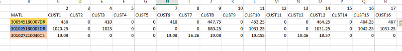
The result will be just the first matching row from each set displayed, as shown in this screenshot from my working on your example excel file:
I have attached the updated Excel file which does the needful for you to review.
Thanks!
EE-Question_Solved.xlsx
- Create a second worksheet
[list=3]On the second Sheet, highlight the column with the materials names in it, and on the data ribbon select "Remove Duplicates"[/list]
This will leave you a list of exactly 1 unique material for each you are desiring to see results.
Now we use a simple vLookup, since it will always pick the first match it encounters.
Assuming your new materials column is Column B on sheet 2, make sure there is an additional line above the headers line. So MATL will appear on "B2"
Then Enter this into Column C: on sheet 2:
=VLOOKUP($B3,EE!$E:$U,C$1,0)On the top column above the Labels number them 1 through 17, so the lookup goes to the correct column
Then drag the formula across to the last "CUST16" column, filling them all, and you can flash-fill down the remaining rows.
The result will be just the first matching row from each set displayed, as shown in this screenshot from my working on your example excel file:

I have attached the updated Excel file which does the needful for you to review.
Thanks!
EE-Question_Solved.xlsx
Make a backup copy of your spreadsheet
Press F11 on the keyboard
In the menu bar click insert then new module
Paste this macro code in the window that pops up
Run the macro (see the menu bar at the top or press F5 while your cursor is still somewhere in the Macro)
Press F11 on the keyboard
In the menu bar click insert then new module
Paste this macro code in the window that pops up
Run the macro (see the menu bar at the top or press F5 while your cursor is still somewhere in the Macro)
Option Explicit

Sub DeleteRows()
Dim r As Range
Dim lngLastRow As Long
Dim i As Long
Dim ws As Worksheet
Dim colKeep As Collection
Dim colDiscard As Collection

Set colKeep = New Collection
Set colDiscard = New Collection
Set ws = ThisWorkbook.ActiveSheet
Set r = ws.Range("E2")
lngLastRow = ws.Range("E1048576").End(xlUp).Row

'collect lines to keep and lines to discard
Do While r.Row <= lngLastRow
On Error Resume Next
colKeep.Add r, r.Text
If Err.Number Then  'only first row containg MATL number is kept
colDiscard.Add r
Debug.Print Err.Number & " " & Err.Description

End If
On Error GoTo 0
Set r = r.Offset(1, 0)
Loop

'discard unwanted lines starting from the bottom
For i = colDiscard.Count To 1 Step -1
Set r = colDiscard(i)
r.EntireRow.Delete
Next i


End Sub
Or the easiest approach would be to use the inbuilt feature to remove the duplicates which is available under Data Tab and called Remove Duplicates.
Please watch this short demo.
RemoveDuplicates.mp4
Please watch this short demo.
RemoveDuplicates.mp4
ASKER
Thanks, All. The answers all worked, but Subodh was first and the simplest. Thanks again for broadening my understanding.
You're welcome! Glad we could help. :)