Multiple criteria to pull in multiple matches on different rows using MATCH, INDEX and SMALL in an Array
I am looking for a formula that will allow me to lookup multiple criteria and pull in multiple matches. For example: My column headers are years, i.e. 2007, 2008, etc. My row headers are the different project types, i.e. New, Old, In Queue, etc. I also have 2 static combo boxes that correspond to City and State, which should also be part of the criteria and as the different city and state values from the drop-down change, the matches should changes as well. I know how to use MATCH and INDEX for multiple criteria for a single match, but I need to match multiple criteria to pull in multiple matches and pull the matches in on separate rows if there is more than one match. I understand that I can use SMALL, but I've been playing around and have not been successful. I would appreciate any assistance with the array formulas that you can provide. Thanks!
I've attached a sample workbook with a matrix of how I want it to look, as well as a sample data tab where the data should come from.
Sample-Workbook-Matching-Multiple-C.xlsx
I've attached a sample workbook with a matrix of how I want it to look, as well as a sample data tab where the data should come from.
Sample-Workbook-Matching-Multiple-C.xlsx
ASKER
Apologies, I know the logic isn't correct, just wanted to give you a visual to back up my written explanation. I will try the formula and get back to you, thanks for the prompt response!
ASKER
Also, per my original question, will this formulas solve for multiple values with the same criteria and put the values on different rows? Or will it pick only the 1st value? I see that you did not use the SMALL function in your formula that I've seen in other solutions. Thanks.
ASKER
Just tried it, it didn't work for any of the cells. Unfortunately, Everything returns N/A. Also, not sure why you are referencing the lookup values off to the right in Columns O and N in the index portion?
based on your example that you attached.
It is not return of multiple values, it is multiple match and return of single values based on multiple criteria match.
so you have four criteria to match in the table and return only from column NAME of the Data table. your multiple 4 criterias are,
the two dropdowns are two of them and then column A and Row 2 of the simple matrix sheets are the other two criteria.
ASKER
You are partially correct, but sorry, I actually do need a return of multiple values for multiple criteria, even though my data on the example may not be mocked up to reflect that. I don't have time to do a proper mock up and I think you may have misunderstood the example, but if you read my original question it may become clearer to you. That's why I list "New' several times on the list, and 'Old" several time on the list, etc. The worksheet was for illustrative formatting purposes only, but if it's tripping you up, please read my original question.
ASKER
In any event, I also still got N/As, it would seem that at least a few of them might have worked..
ASKER
My real data will have multiple matches for each Action.
you got N/A because you have leading and trailing spaces either in your lookup values or in your tables.
for example look at your sheet Data cell B2 the word New has a trailing space. again, look at your simple matrix sheet cell N1 word Tampa has a trailing space.
For lookup function to work, your data needs to be consistent. we can use trim function to ignore the spaces but then for functional array operation we then need to use unnecessary control +shift+enter key and plus it will make the formula slow as well. so it better to clean up the data before doing any lookup.
Re your comment
My real data will have multiple matches for each Action.the formula I have given you is based on what you have provided as a sample data. if your data structure is other than the one you attached, then i would not know how it is structured.
ASKER
Sorry, I don't know what else to say here, my question clearly articulated what I needed to do. I'm sorry you misunderstood, however I still need my original question answered. My sample data is not contradictory to my question, but if you are indicating that you are unable or unwilling to assist me further, please let me know and I will request moderator assistance for next steps.
ASKER
If you did not get N/As when you tested your formula, please send me your sample workbook and I can piggyback off of that in this thread if someone else jumps in. Thank you for your attempts.
here it is with the trim function included.
attached is the workbook with formula embedded in it.
plz allow me to demonstrate how values you had repopulated in your example cannot be returned by any formula, because you cannot really find any link to it.
so take a look at the example you have given, word def to be returned in B4 which is beneath year F'18 and is Florida and Tampa and Action is New.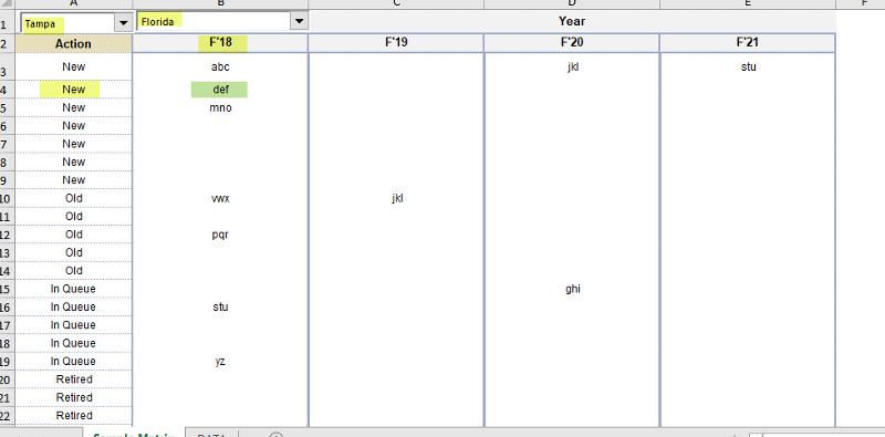
so now, when we look at the actual data, you can see that there this value of "def" but the corresponding columns to it, does not have F18, or Florida or Tampa, they have different values, therefore the lookup formula cannot return anything there.
I am trying to help you, if this does not make any sense, sorry I cannot help any further on this. Perhaps, I am missing something :)
Hope anyone else could be of assistance to you on this.
Sample-Workbook-Matching-Multiple-C.xlsx
ASKER
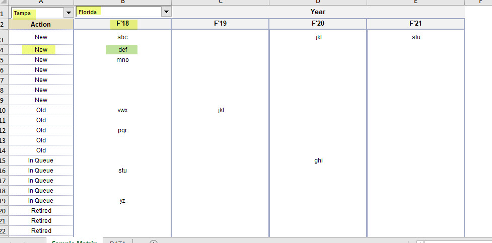
I truly appreciate your help here and I think I understand your concerns :) :-) What you are saying makes perfect sense to me, but let me try to clear this up: I need you to shift your focus off of the sample I provided which I've already acknowledged multiple times will not be accurate and match. It's only an example. Perhaps i should not have attached it and just left my question. What I need you to focus on is my question and to disregard the sample data, but you insist on trying to use the sample data.... we kind of need to think outside of the box here. Ignoring what I provided, my question is, If the data were correct, how would I return multiple values? For example if the criteria were F'18, Tampa, Florida and the Action was New, and values were abc, def, ghi. How would we capture all 3 of these values in different rows under New in F'18? Does that help you?
ASKER
Does this file help better? I took the time to make the example match more with what I'm trying to accomplish.
Sample-Workbook-Matching-Multiple-C.xlsx
Sample-Workbook-Matching-Multiple-C.xlsx
Hi,
again the pre-populated data that you have put there is not correct. becuase you have put the values in the returned cells which does not exist in the table with its corresponding column value.
however, regardless of your example, I have came up with a solution and it is a killed formula :)
please see attached file. you can see in the screenshot for Chicago Illinois , years, and the [progress, complete, pending} whatever data with its corresponding values exists, it returns it. if it does not find it. it will return blank. also the formula is array, so it should be entered with control shift enter.
=IFERROR(INDEX('Sample Data'!$E$2:$E$26, SMALL(IF(COUNTIFS(INDEX(Ma
Sample-Workbook-Matching-Multiple-C.xlsx
ASKER
Thank you again, but sorry, my file is correct with the exception of City and State. I told you that I need to be able to toggle between the City and State on the drop-down, so I couldn't make the values in the returned cells match the City and State on the data file in every instance. Regardless, I believe it's intuitive enough for someone to come up with a formula that will work with any data, not just the exact sample data I provided. This is not helpful because if something changes, on a row, if I have real data, it won't work. Again, thanks for attempting to solve this, but I don't think you are fully understanding what I need to do here.
ASKER
There should not be duplicate entries on each row when the City and State is changed. Each entry is unique or the row should be blank.
Ok. You can ask the moderator to send email to more experts. as far as I know, No-one would be able to produce a formula for the example you have given. Because, simply the data you want to turn does not exist. Look at your example here.
this is what you have described that the end result should look like
A)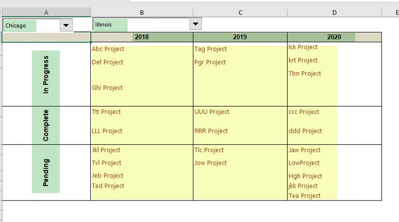
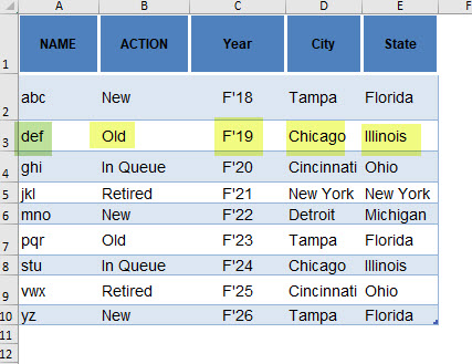
and this is the actual data from which the column E needs to be returned.
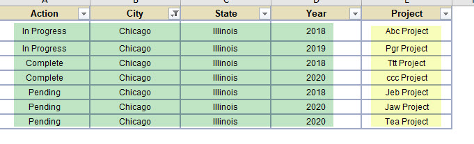
Now, for example where do you see "Ghi Project" under city Chicago state Illinois? it does not exist, if it does not exist, how would you return it there?
Sorry, cannot help any further on this. because it is simple not possible what you are asking based on the example given.
this is what you have described that the end result should look like
A)

and this is the actual data from which the column E needs to be returned.
Now, for example where do you see "Ghi Project" under city Chicago state Illinois? it does not exist, if it does not exist, how would you return it there?
Sorry, cannot help any further on this. because it is simple not possible what you are asking based on the example given.
My last attempt.
Please see two attachments.
A) Example A which is the one based on the logic of including the City and State.
B) Example B which is based on the logic of excluding the CIty and state and it will return exactly as you asked.
EXAMPLE-B.xlsx
EXAMPLE-A.xlsx
Please see two attachments.
A) Example A which is the one based on the logic of including the City and State.
B) Example B which is based on the logic of excluding the CIty and state and it will return exactly as you asked.
EXAMPLE-B.xlsx
EXAMPLE-A.xlsx
ASKER
Example A is correct! Give me a few hours to test on my real data, but I believe this is what I need! Thank you!
ASKER CERTIFIED SOLUTION
membership
This solution is only available to members.
To access this solution, you must be a member of Experts Exchange.
if your logic in the data were correct, then this is the formula you could have used to be placed in B3 and then dragged/coped to the right and down.
=LOOKUP(2,1/(Table1[State]