formula to reduce values to a predetermined range of numbers

The sample provided does not explain what you are trying to achieve. Please explain further with examples and why a particular number goes to the result.

Hi Rob,
Maybe it cannot be done.
The simple explanation is to allocate a value of one to the lowest number in the range and a value of 100 to the highest value in the range,
The two samples provided show that.  Then via formulas if there is such a thing to smooth out values proportionately to other sells in the range.
I'm almost convinced now it cannot be done.
Please put me out of my misery and tell me so
Thanks

It should be doable, I think the tricky part is getting the lowest value to be 1 (rather than 0) and the highest value to be exactly 100.

I'll play around with it in a bit if you don't have a solution by then...

(Are you actually a professional racer? )

---

»bp

Hadn't realised that the sample was actually two examples, even so still wasn't clear.

However, to allocate 100 to highest and 1 to lowest then try this formula in F3:

=IF(E3=MAX($E$3:$E$6),100,IF(E3=MIN($E$3:$E$6),1,"XXX"))

Copy down through rows 4 to 6

Not sure what you mean by smoothing out the values in between, what would you expect the results to be in the samples? When explained, this would replace the XXX part of the above formula.

Could the lowest/highest numbers occur more than once? If so, what should be done with them?

Yes Bill I'd like to think I was a pro but haven't made a penny yet :)
Making the lowest value a zero may still be okay for my purpose.

Rob, that formula does fish out the highest and lowest numbers not sure how to handle the remaining numbers. Perhaps as Bill suggested a zero for the lowest value may be the way around it.

Until we know how you want the in between numbers handled then we can't progress any further.

However, a suggestion of how you might want is below:

=ROUND(E3/(MAX($E$3:$E$6)-MIN($E$3:$E$6))*100,0)

This compares MAX and MIN of the range to get a value for the range of numbers, sample 1 is 1000000 - 22 = 9999978

Then each of the other numbers is divided by that number and multiplied by 100 to get its equivalent value between 1 and 100, rounded to zero decimal places.

So example 1 would give:

10000000      100
4444444            44
333333            3
22                  1

Using the same method, the results on the second sample go awry because of the range of values 356 to 1666889, a range of 1666533 so 356 as a proportion of that range is much smaller; when rounded goes to zero.

Looks good Bill, I'll run with that one. Thanks to Rob too.
Cheers
Ian

Okay, I think I like this version slightly better, it's a little truer to the math involved and should hold up better on ranges with smaller numbers, etc...

Number-reduction.xlsx

---

»bp

Okay, I think I REALLY have it now :-)

Number-reduction.xlsx

---

»bp

Okay I will use that one, thanks and I forgot to ask can you add indexing to it using col C as the index.  see attached  thanks
Number-reduction.xlsx

I don't understand what you mean by "indexing" ?

---

»bp

Looks impressive Bill, would you mind adding the Index formula to that one. I will copy this down for 50,000 rows or more

The sample I included had 2 or 3 series of bets each series is numbered, Race 1 may have 8 starters r2 10 starters etc.
I need an index to distinguish where a series starts and ends

Okay, see if this is what you were thinking.  Notice that the formula now is an arrau formula, so if you eidt it you have to press CTRL-SHIFT-ENTER to save that formula.  Also, I am letting it match on all of columns C and E.  If you notice any delays during recalc you could limit those ranges in the formula to the specific first and last row of used data, but this seemed easier for now.

The array formula I used is:

{=ROUND((((E3-MIN(IF(C:C=C3,E:E,10^10)))*(100-1))/(MAX(IF(C:C=C3,E:E,-1))-MIN(IF(C:C=C3,E:E,10^10))))+1,0)}

Select allOpen in new window

As demonstrated in this workbook:

Number-reduction--4-.xlsx

---

»bp

Hi Bill,
I'm not sure this is working for me. As I have closed the question perhaps the correct protocol is to open a new one.
I hope you don't mind me posting your earlier formula and request it to be modified to include indexing or an INDIRECT
function I think it may be.

Not a problem.  Did you look at the attached workbook, that isn’t what you wanted?

Sorry, I hadn't but now have. The problem with arrays they are not workable when using tens of thousands of rows.
They take a long time to calculate.

Ian,

A couple of thoughts on this:

1. Would you be open to a VBA macro approach to implement a user defined function that could then be used in the worksheet?  We could avoid the complex indexing or array type formula this way and have something very simple as the worksheet formula, and then do all the heavy lifting (more efficiently and understandably) in the VBA UDF.
2. Are the same values in the "grouping column" (where you had value groupings of like 100, 120, 150 etc) all contiguous for a grouping value?  Meaning would all the 100's be together, and all the 150's, etc?  Or can they be spread around and interspersed?

---

»bp

Hi Bill, been a busy day again but will look at this tomorrow, I have an idea of adding a function that indexed perfectly for another worksheet I use.
I will send to you for your expert opinion.
Thanks again.

Okay, let me know how it goes.

---

»bp

Have a look at this formula which is yours plus an added indirect function to link two helper columns to speed up the calcs.
However needs adjusting as explained in sheet. Thanks/Cheers.
Number-reduction--4-.xlsx

Have a look at this formula which is yours plus an added indirect function to link two helper columns to speed up the calcs.

Okay, so that seems to imply that the answer to one of my earlier questions is "YES, they are contiguous"?  I didn't want to make that assumption until it was stated...

---

»bp

They can be anywhere in the series. No grouping.  Series meaning one race same as in example I gave, the 100 could be anywhere.

Well, if they are all contiguous for a certain value, then I don't see how the example you posted last helps.  As in the attached test case, notice the 100 group is wrong when it isn't contiguous.

Number-reduction--4-.xlsx

---

»bp

The part of the formula I was more interested in was the INDIRECT function and used for recognising beginning and ending of each series.
Plus the linkage to the two right hand columns which help speed up the calculation. If you can modify the other bits like MAX etc as that is wrong.

I must be missing something.  The technique used to calculate those two right hand columns with the start and end rows of a series aren't valid, since you confirmed "They can be anywhere in the series. No grouping.  Series meaning one race same as in example I gave, the 100 could be anywhere."  Based on that statement the technique used in your example is not valid since it relies on contiguous elements in a series.

---

»bp

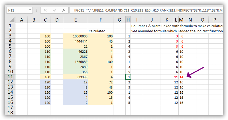
I've ranked them using the formula in column H. This interacts with columns L&M to speed up calcs.
If you know of a way to display value instead of Rank or use column H as a helper column.
Number-reduction--5.xlsx

That illustrates the problem I'm talking about.

Notice cell H11 with the formula:

=IF(C11="","",IF(E11=0,0,IF(AND(C11=C10,E11=E10),H10,RANK(E11,INDIRECT("$E"&L11&":$E"&M11),0))))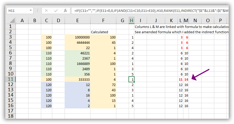

Select allOpen in new window

That isn't grouping that row which is part of series with 100 in column, rather it is grouping it with rows 11 to 14 (see below) which isn't correct).

---

»bp

OH........ how did row 11 get sorted ? Column C is wrong as you can see by the orange background.
Column C is the index column and is static..
I've corrected it and is attached.
Number-reduction--6.xlsx

So then, all the 100 rows WILL ALWAYS be together?

---

»bp

those are indexes for example
Race 1
Race 1
Race 1
Race 1
Race 2
Race 2
Race 2
Race 3
Race 3
Race 3
etc

Thanks Bill, I'll take a look after some sleep

Sorry Bill was away most of the day visiting a friend in hospital a long way away.
Yes the formula does work and calculates quite fast on my i9 64GB 2TB computer.
Thanks Bill for your patient help on this one and no doubt see you on EE again soon.
Ian

That's great Ian, glad that was useful, thanks for the feedback.

---

»bp