excel 2016 - custom formatting
Hi experts, could you please help me change the following cell formatting under the;
format cells/ number/ custom
[Red]+0.00;[Blue]-0.00;[Bl
- basically if col "c" = col "d" then show tick in blue, otherwise show col "d" in red
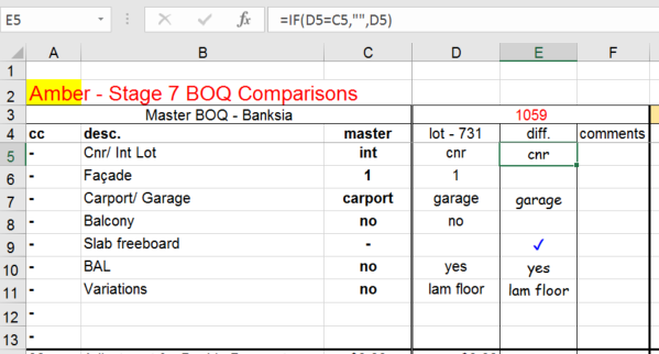
- the formula i have in column e is =IF(D5=C5,"",D5)
format cells/ number/ custom
[Red]+0.00;[Blue]-0.00;[Bl
- basically if col "c" = col "d" then show tick in blue, otherwise show col "d" in red
- the formula i have in column e is =IF(D5=C5,"",D5)
ASKER
thanks ryan, but im looking for a solution under the 'custom formatting'as per my question, using the blue tick, etc.
you could try this:
[Red]+0.00;[Blue]-0.00;[Blue]"✔";[Red]GeneralASKER
hi ryan, no does not work, i have attached worksheet & hilited in yellow the cells that show you the problems with the formula & custom format.
comparison_spec-formula-errors.xlsx
comparison_spec-formula-errors.xlsx
AFAIK Custom format cannot include a formula comparison so the check for the two cells being equal will have to be done elsewhere.
Conditional Formatting can have the formula to check the cells being equal.
Conditional Formatting can have the formula to check the cells being equal.
The issue on your file in row 6 is the values in C6 and D6 may look the same as the number 1. However, C6 is a number but D6 is text.
If you change the formula to:
=IF(C6*1=D6*1,"",D6)
This will allow for the values in C or D being text and multiplying by 1 will force excel to re-evaluate the cell contents and will recognise it as a number.
The values in this case are then equal so result is "", however, your Custom Format is applying the tick to zero values not blank so change the formula to:
=IF(C6*1=D6*1,0,D6)
But that doesn't allow for genuine text entries like row 7, try this instead:
=IF(IF(ISNUMBER(C6*1),C6*1
ASKER
hi rob, which cell/s do i put in your last IFSTATEMENT?
Slight change after taking another look:
=IF(D6="","",IF(IF(ISNUMBE
This would go in E6 but can then be copied to populate all of the formulas in columns E, H, K, N etc as per attached
comparison_spec-formula-errors--1-.xlsx
=IF(D6="","",IF(IF(ISNUMBE
This would go in E6 but can then be copied to populate all of the formulas in columns E, H, K, N etc as per attached
comparison_spec-formula-errors--1-.xlsx
I believe you can simplify Rob's formula to:
=IF(D5="","",IF($C5 & "" = D5 & "",0,D5))ASKER
hi byundt after pasting in your formulas, the results do not pick up any cell formatting whereas robs do..
ASKER CERTIFIED SOLUTION
membership
This solution is only available to members.
To access this solution, you must be a member of Experts Exchange.
ASKER
thats funny, when i pasted your formula only the values updated not the formatting, ie the tick, red font, etc..ok thankyou
ASKER
thankyou experts for your solutions
Conditional Formatting
https://www.excel-easy.com/data-analysis/conditional-formatting.html