Help in Excel to get the TOTAL counts based on the month & year and its AVERAGE
Hello... very frustrating but hope an expert can help.
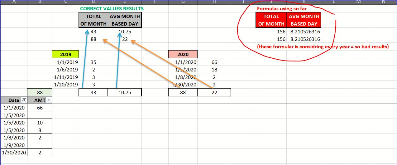
I am trying to get the total days of a month of a specific year.
Also the average of said month based on days found with value.
So based on the image below:

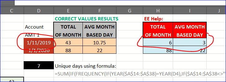
I filter only data from jan 2020. The values should as displayed in green columns: 88 counts and avg. 22% (note that some says have no values, I don';t want to count those).
Yet in the formula used, it reading all January no matter what year.
So I am missing how to set the formula to identify the year I want.
Help?
(also included the excel so u guys can play with the values maybe I have those data wrong)
CalcMonthBasedYear.xlsx
I am trying to get the total days of a month of a specific year.
Also the average of said month based on days found with value.
So based on the image below:
I filter only data from jan 2020. The values should as displayed in green columns: 88 counts and avg. 22% (note that some says have no values, I don';t want to count those).
Yet in the formula used, it reading all January no matter what year.
So I am missing how to set the formula to identify the year I want.
Help?
(also included the excel so u guys can play with the values maybe I have those data wrong)
CalcMonthBasedYear.xlsx
Which version of Excel are you using? I ask, because Excel 2016 on an Office 365 subscription just introduced some new functions that make this kind of problem easy.
I put the months January through December in cells R2:R13 and the year in cell S1. Formulas for sum of AMT, number of days in that month with an AMT and average for that month are given by:
I put the months January through December in cells R2:R13 and the year in cell S1. Formulas for sum of AMT, number of days in that month with an AMT and average for that month are given by:
=SUMPRODUCT((YEAR($A$14:$A$38)=S$1)*(MONTH($A$14:$A$38)=MONTH($R2 & " 1"))*$B$14:$B$38)
=COUNT(UNIQUE(FILTER($A$14:$A$38,($B$14:$B$38<>"")*(YEAR($A$14:$A$38)=S$1)*(MONTH($A$14:$A$38)=MONTH($R2 & " 1")),FALSE)))
=IFERROR(S2/T2,"")
In case you don't have Excel 2016 on an Office 365 subscription, you can count the number of unique days in the month with an AMT by adding an auxiliary column to the data table. The auxiliary column tests whether there is an AMT in column B. If so, if copies the date from column A. If not, it returns January 1, 9999 as the date.
=IF([@AMT]="",DATE(9999,1,1),[@Date])          'Copied down in C14:C38
=SUMPRODUCT((YEAR($C$14:$C$38)=Z$1)*(MONTH($C$14:$C$38)=MONTH($R2 &" 1"))/COUNTIF($C$14:$C$38,$C$14:$C$38))
One complication that you have with the January data is the two entries for 5 Jan. When doing an average Excel will count this as two entries so is dividing the total of 88 by 5 to give 17.6 rather than your expected division by 4 to get 22
I have overcome this by adding a helper column to your data which sums each day and used Subtotal to put average at top the column.
I have also used a Pivot Table (on separate sheet) to show the sum and average figures.
See attached.
CalcMonthBasedYear.xlsx
I have overcome this by adding a helper column to your data which sums each day and used Subtotal to put average at top the column.
I have also used a Pivot Table (on separate sheet) to show the sum and average figures.
See attached.
CalcMonthBasedYear.xlsx
ASKER
I think all the answers are great, but maybe I left out a necesary data (somehow erased while doing the Excel): the dates columns (see below column 'C') - if u notice the calcs in columns J and K, both are pointing to these cells (but I leftr it empty by mistake)
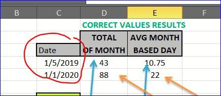
The data in column D and E are constant I entere to show the result I am trying to get.
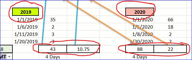
The data under 2019 and 2020 (see below), is just my calculations calculations in order to place the constant values on columns D and E
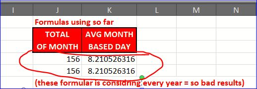
The failed formulas I am using and want tocorrect are located in column J and K (see below).
The help I am looking for is how to fix these 4 formulas to calculate TOTAL/MONTH and AVERAGE/MONTH per YEAR requested.
Based on what I said here, are all the recommnedations the same?
The data in column D and E are constant I entere to show the result I am trying to get.
The data under 2019 and 2020 (see below), is just my calculations calculations in order to place the constant values on columns D and E
The failed formulas I am using and want tocorrect are located in column J and K (see below).
These failed formulas reads the column "C" dates to get the month
Total Month 2019 =SUM((MONTH(A14:A38)=MONTH(C4))*B14:B38)
Total Month 2020 =SUM((MONTH(A14:A38)=MONTH(C5))*B14:B38)
Average Month 2019 =SUM((MONTH(A14:A38)=MONTH(C4))*B14:B38)/SUM(IF(MONTH(A14:A38)=MONTH(C4),1))
Average Month 2020 =SUM((MONTH(A14:A38)=MONTH(C5))*B14:B38)/SUM(IF(MONTH(A14:A38)=MONTH(C5),1))
The help I am looking for is how to fix these 4 formulas to calculate TOTAL/MONTH and AVERAGE/MONTH per YEAR requested.
Based on what I said here, are all the recommnedations the same?
See updated file attached.
Used SUMIFS function in K4:
=SUMIFS($B$14:$B$38,$A$14:
AVERAGEIFS function in L4:
=AVERAGEIFS($C$14:$C$38,$A
Still had to use the helper column for the average so that it counts the occurrences with multiple values on one day as one occurrence.
CalcMonthBasedYear.xlsx
Used SUMIFS function in K4:
=SUMIFS($B$14:$B$38,$A$14:
AVERAGEIFS function in L4:
=AVERAGEIFS($C$14:$C$38,$A
Still had to use the helper column for the average so that it counts the occurrences with multiple values on one day as one occurrence.
CalcMonthBasedYear.xlsx
ASKER
Can u explain a bit the ">=" and "<="
ASKER
Sorry... had to unmark as solution... when I applied your formulas I got wrong values and it's because u added the "AMT2" which my excel don't have.
Is there a way to get these values without this additional column?
(the reason is because the real live excel has over 15 columns I need those 2 values with, and if I use your formula, I have to add 15 more columns)
Is there a way to get these values without this additional column?
(the reason is because the real live excel has over 15 columns I need those 2 values with, and if I use your formula, I have to add 15 more columns)
D4 is a date representing the first of a month. You are looking for entries in column A that are in the same month.
>= means "greater than or equal to" that date, ie on or after the first of the month.
EOMONTH(D4,0) then converts that date to a date for the end of the month.
<= means "less than or equal to" the month end date ie on or before the end of the month.
That then gives dates that are in the same calendar month.
As mentioned earlier, the issue with the data is multiple entries on the same day increasing the count for the month to calculate the average.
ASKER
Thac for the explaination on your entry.
But to use "AMT2" column I have to created additional 15 columns.
Will keep trying to find
But to use "AMT2" column I have to created additional 15 columns.
Will keep trying to find
I have come up with a way round it. Can you upload a file with all 15 amount columns?
I am looking at using Pivot Table to summarise by year, month and day. This will consolidate the amounts where there are multiple entries on a day.
Then using SUMIFS and AVERAGEIFS on the Pivot Table rather than source data, AVERAGEIFS can use a criteria to exclude days with blank value.
I am looking at using Pivot Table to summarise by year, month and day. This will consolidate the amounts where there are multiple entries on a day.
Then using SUMIFS and AVERAGEIFS on the Pivot Table rather than source data, AVERAGEIFS can use a criteria to exclude days with blank value.
ASKER
I really want to use a formula, no pivot table nor VBA no additional columns (unless totally necessary).
That said, I did find a way that we could this: counting the unique dates with the column of the year.
(why counting the dates of that month/year? to use it in the division to get the average)
I tried this formula:
=SUM(IF(FREQUENCY(IF(YEAR($A$14:$A$38)=YEAR(D4),IF($A$14:$A$38<>"",MATCH($A$14:$A$38,$A$14:$A$38,0))),ROW($A$14:$A$38)-ROW($A$14)+1),1))
But can't get it to seperate the month.
(still looking)
What do u think?
How about just one helper column to the left of the dates???
See attached. Column A looks at the dates to see if it is repeated with a value in columns C to Q (15 values). If it is unique, it returns 1 otherwise returns 0. The AVERAGE then uses the sum of this column with relevant date range to determine a count of unique dates.
CalcMonthBasedYear.xlsx
See attached. Column A looks at the dates to see if it is repeated with a value in columns C to Q (15 values). If it is unique, it returns 1 otherwise returns 0. The AVERAGE then uses the sum of this column with relevant date range to determine a count of unique dates.
CalcMonthBasedYear.xlsx
Would you be willing to store your file on OneDrive (either Business or Personal) and access it using a web browser? If so, you would be using Excel Online, and would have access to the new UNIQUE and FILTER functions. You could then use the formulas I suggested in my very first Comment and example.
There would be no VBA, no PivotTable, no auxiliary columns. Just working formulas returning the desired results.
I stored the sample file in the Public folder of my Personal OneDrive. You may access it at https://1drv.ms/x/s!AoHfCiwUeT98shL7rZwWlZ_9vcza?e=EX4Oyc
There would be no VBA, no PivotTable, no auxiliary columns. Just working formulas returning the desired results.
I stored the sample file in the Public folder of my Personal OneDrive. You may access it at https://1drv.ms/x/s!AoHfCiwUeT98shL7rZwWlZ_9vcza?e=EX4Oyc
ASKER
Hi Byndt... unfortunately, my supervisor hasn’t authorized it (not even to our own OneDrive).
Right now I am working with Rob recommendation to assure accommodate the needs.
Right now I am working with Rob recommendation to assure accommodate the needs.
ASKER
Hi Rob,
Just went over the Excel and filled out the 14 columns with value and results changed (see I4 changed to 8.6 instead of 10.75, considering 'blank' cells - in the sheet 'ORIGINAL' I placed how I calculated the "CURRENT VALUES RESULTS)
I noticed that it's not considering the AMTx columns when there is NO-VALUE.
If I use 'Date Check" column, I'll have to use it for the 15 columns because some cells are blank.
I placed the formula '=SUM(IF(FREQUENCY(IF(YEAR
(I have attached the excel with you formulas and additional column data and a "SUMMARY" area to double-check the values)
Any other way we can work around this?
Thinking about it, my suggestion with identifying unique dates falls down when there are multiple value columns.
A particular date could have a value for one account so should be counted in the average but doesn't have a value for another account so should be ignored.
Back to the drawing board!!
A particular date could have a value for one account so should be counted in the average but doesn't have a value for another account so should be ignored.
Back to the drawing board!!
ASKER
Ooops! forgot the excel
CalcMonthBasedYear--wEE-.xlsx
CalcMonthBasedYear--wEE-.xlsx
ASKER
I was thinking maybe counting the AMTx columns who has NO-VALUE and subtracting from UNIQUE DAYS counted, that me give a correct of days?
WHat u think?
WHat u think?
ASKER
I think if a formula wuere it would count the unique days of the month, not adding the other years, then counting the BLANKS, then that value can be used to get the average:
Example:
Total = 43
Counted = 5
Blank = 1
Average = 43 / (5-1)
What u think?
(need the formula)
Example:
Total = 43
Counted = 5
Blank = 1
Average = 43 / (5-1)
What u think?
(need the formula)
ASKER
Well, I got the count the blanks:
=COUNTBLANK(C11:C35)
But how to included based on the DATE entered.
=COUNTBLANK(C11:C35)
But how to included based on the DATE entered.
With your summary area getting Total and Average for a particular month, are you looking at only one account at a time, ie only AMT1 or only AMT3?
ASKER
The summary area was for validation only on the formula.
The end result is to come up with the formula and have at top as is in the excel. The user will click on the date and change it and the formula will get thr year/month and set its results.
The end result is to come up with the formula and have at top as is in the excel. The user will click on the date and change it and the formula will get thr year/month and set its results.
ASKER
Note, I placed 2 vales 1/1/2019 and 1/1/2020 just to have 2 years, but it will be 1 cell for the user to enter his/hers date.
I believe I can reduce the number of auxiliary columns to 1 by using a Data Table. But I will need to know the details of the layout and desired report, because each reported value will be a column (or row) of results in the Data Table.
In essence, the Data Table will be plugging the numbers 1 through 15 as an input into an INDEX formula that selects one of the AMT columns. A 1 selects the first AMT, a 2 selects the second, and so on. I would then use the formulas already posted to return the sum, count of unique days in the month & year, and average.
The reason I need the layout is to plug in the month(s) and year(s) that you want reported. If you need to have months listed in a single column and years in a single row (a 2D table), then I would need to use two Data Tables: a 1D data table for the 15 different AMT and a 2D data table for the months and years. Note that 2D data tables may only report a single value, so if you need sum, unique days and average, you would need three 2D data tables.
So are you intending to place the Total and average formulas for each column of data? Like the SUBTOTAL function you have above AMT1 column.
The process that I am looking at also uses a Data Table (rather than standard list/range) and will have 2 user inputs,
1) the account for which they want the Total & Average
2) the 1st of the month which they are looking at.
This still has only one helper column to check the unique dates but based on the User Input it will use the relevant column (Account) to check for blank values.
1) the account for which they want the Total & Average
2) the 1st of the month which they are looking at.
This still has only one helper column to check the unique dates but based on the User Input it will use the relevant column (Account) to check for blank values.
See attached.
Date Inputs in D4 and D5 as before.
Dropdown selection in D3 to choose Account header (linked to row 10 Table headers)
Column A date check will change based on the Account selection to determine if the relevant row for the chosen account is blank and whether the date is unique.
Column A is then used as the SUMIFS in the Average calculation to get a count with which to divide the total to get an average.
CalcMonthBasedYear--wEE-.xlsx
Example of Data Table
CalcMonthBasedYear--wEE-.xlsx
CalcMonthBasedYear--wEE-.xlsx
ASKER
Hi byundt,
The layout is just like the original excel pr the last excel I sent with the exception that the results is to be laced on H4 for (total of month) and I4 (for average of that month). The user interface is the cell D4 so they can enter the date. Then the formula would read the date and place results on H4 and I4 accordingly.
What I need is to display end result on H4 and I4
ASKER
Rob, the only data that will change is:
cell D4 = the user enters a date
cell H4 = displays the total of that month based on the date entered in D4
cell I4 = displays the average of that month based on the date entered in D4
I ran your excel and when I change D4 to '1/11/2019', instead of giving the same result because is the same month and the year, it gives a different result (see below).
Just to check, is that 1 November 19 or 11 January 19?
My file has assumed entry of First of the month. I can change it so that any date entry will be rounded back to first of the month.
My file has assumed entry of First of the month. I can change it so that any date entry will be rounded back to first of the month.
ASKER
No, '1/11/2019' uses US standard MM/DD/YYYY, do its January 11, 2019.
I can extract the year (=YEAR(x)) and month (MONTH(x)), it just placing that within the formula that has gotten difficult.
I can extract the year (=YEAR(x)) and month (MONTH(x)), it just placing that within the formula that has gotten difficult.
ASKER CERTIFIED SOLUTION
membership
This solution is only available to members.
To access this solution, you must be a member of Experts Exchange.
ASKER
Yes! Thank u much! I can work with this formulas!!!! Definitely the 'Date Check' column is needed (I would like not to use but it seems its a must)
ASKER
I know its closed, but q question:
In column 'Date Check', the formula '=IF(INDEX($C11:$Q11,MATCH(
(Your feedback super valuable on this)
In column 'Date Check', the formula '=IF(INDEX($C11:$Q11,MATCH(
(Your feedback super valuable on this)
Sorry, can't comment for definite on why that is slow to calculate.
I am aware of some functions being what is called "volatile" which means they will recalculate every time the sheet recalculates rather than only if the cells to which it refers recalculates.
I went with using a Data Table to avoid using whole column references which are known to cause slow calculations.
ASKER
Thanx!
(still testing)
(still testing)
To speed up calculation, it would be worth considering using Pivot Table, don't know why you are averse to doing so.
See attached.
Count & Average (2) has a different calculation in column A which will hopefully be quicker to calculate. That sheet is now purely data, add the remaining data and ensure that it is included in the Table boundaries. Bottom right corner of the existing table is a cell marker, you can drag this to include the new data rows. Alternatively, put the cursor anywhere in the data table and there will be an extra header on the Data ribbon for Table Tools. On the left hand end there is an option to Resize Table, click that and select the data or amend the row value manually.
The pivot sheet is now where the calculations take place.
Select the Account in I2. Right click on the Pivot Table in columns A to D and select Refresh. The values in the pivot will change and the calculations will update, hopefully with no noticeable time delay.
CalcMonthBasedYear--wEE-.xlsx
ASKER
Thanx!
Very helpful!
Very helpful!
SOLUTION
membership
This solution is only available to members.
To access this solution, you must be a member of Experts Exchange.
ASKER
Hi, make sense and its something I gonna incorporate, Thanx!
You can loop through the Excel seeet to get count per given relevant month.
https://support.microsoft.com/en-us/help/142126/macro-to-loop-through-all-worksheets-in-a-workbook