Value Filter Top Ten not working correctly.
Dear Experts:
I got a pivot table with a Sales Value Field showing values for 2020 and 2021.
I am showing the 2021 sales values as difference from the 2020 values (Diff-2021-2020).
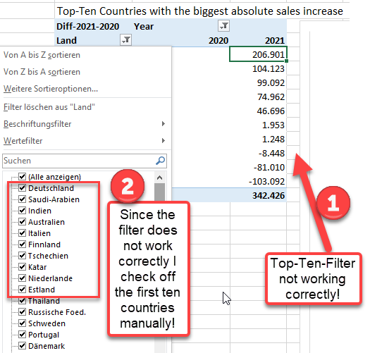
If I perform a Top Ten Value Filtering on the country filed, the filter does not work correctly.
The value top ten-Filter shows:

But actually the top 10 Filter should show ...

Is this a known bug or am I doing something wrong??
Or could somebody come up with a macro code that produces the correct result?
I have attached a sample file for your convenience.
Help is very much appreciated. Thank you very much in advance.
Regards, Andreas
EE-top-10-items-not-working-correctly.xlsm
I got a pivot table with a Sales Value Field showing values for 2020 and 2021.
I am showing the 2021 sales values as difference from the 2020 values (Diff-2021-2020).
If I perform a Top Ten Value Filtering on the country filed, the filter does not work correctly.
The value top ten-Filter shows:
But actually the top 10 Filter should show ...
Is this a known bug or am I doing something wrong??
Or could somebody come up with a macro code that produces the correct result?
I have attached a sample file for your convenience.
Help is very much appreciated. Thank you very much in advance.
Regards, Andreas
EE-top-10-items-not-working-correctly.xlsm
I also get the expected results in Excel 2010. Did you try right clicking the table then selecting "Refresh"? What version of Excel are you using? I have often seen weird results that become normal after rebooting my machine so you might try that.
ASKER
Dear both,
thank you very much for your quick help.
I inadvertently sent you the Pivot Table with the correct results, i.e. I had checked the first 10 items manually after I detected that the Top-10-Filter did not work. I am sorry I should have sent you the right file right away.
Now pliease find attached the file with the Top-Ten-Filter not working correctly.
I am pretty sure this is a bug.
It would be great if you could come up with a macro solution.
Help is very much appreciated. Thank you very much in advance.
Regareds, Andreas
EE-top-10-items-not-working-correctly.xlsm
I think I have a lot to learn from this question, and I hope I can help you a little bit at the same time.
You are using features I don't quite understand, but I made a small bit of progress.
When I don't understand a pivot table problem, I like to simplify things as much as possible.
I am attaching ee2.xlsx which is greatly simplified but still duplicates your problem.
The data source was simplified as follows.
I deleted vba.
I sorted it by Land, Category and year.
I converted the formulas into constants.
I deleted all the hidden worksheets.
I deleted all the columns that were unrelated to our problem.
I deleted all Lands except the Correct top 10 plus a few extra from the incorrect top 10.
I copied your pivot table (PT_AbsDiff) to my own version (BobsPivot) which was linked to the same slicer.
After simplifying the data source, a refresh the AbsDiff top 10 table still shows exactly the same wrong item.
I then did the following.
I cleared BobsPivot by unchecking all fields in the field list, and removing the filters.
I rebuilt BobsPivot to match yours but got completely different results which you can see below and in EE2.xlsx
 That huge difference did not surprise me because your pivot table used Calculated Items to “zero out” 2020 and replaced 2021 with a SalesIncrease of 2021 minus 2020.
Alt JtJL shows these Calc Items:
But, when I deleted these Calculated Items I expected to see your AbsDiff table fall apart because I thought I had removed the “zero out” ability
But after refreshing, NOTHING HAD CHANGED in your table
I now realize that you are not using Calc Items to zero out 2020, and you must be using some other magic.
In fact, I simply cannot make BobsTable look like your AbsDiff table.
Can you teach me how you did it? I think this "other magic" is related to your weird results in the top 10 selection.
Rberke(aka UncleBob)
P.S.
You question hits me in my weak spot. I have hardly ever use Calculated Items because they have a VERY annoying habit of screwing up subtotals. For instance in the follow hypothetical case all of the red and blue cities are totaled twice, but the tossup city is only totaled once.
You are using features I don't quite understand, but I made a small bit of progress.
When I don't understand a pivot table problem, I like to simplify things as much as possible.
I am attaching ee2.xlsx which is greatly simplified but still duplicates your problem.
The data source was simplified as follows.
I deleted vba.
I sorted it by Land, Category and year.
I converted the formulas into constants.
I deleted all the hidden worksheets.
I deleted all the columns that were unrelated to our problem.
I deleted all Lands except the Correct top 10 plus a few extra from the incorrect top 10.
I copied your pivot table (PT_AbsDiff) to my own version (BobsPivot) which was linked to the same slicer.
After simplifying the data source, a refresh the AbsDiff top 10 table still shows exactly the same wrong item.
I then did the following.
I cleared BobsPivot by unchecking all fields in the field list, and removing the filters.
I rebuilt BobsPivot to match yours but got completely different results which you can see below and in EE2.xlsx
That huge difference did not surprise me because your pivot table used Calculated Items to “zero out” 2020 and replaced 2021 with a SalesIncrease of 2021 minus 2020.Alt JtJL shows these Calc Items:
'PerCentage Change 2020/2021' =IF('2020'=0,0,('2021'-'2020')/'2020')
SalesIncrease ='2021'-'2020'
But, when I deleted these Calculated Items I expected to see your AbsDiff table fall apart because I thought I had removed the “zero out” ability
But after refreshing, NOTHING HAD CHANGED in your table
I now realize that you are not using Calc Items to zero out 2020, and you must be using some other magic.
In fact, I simply cannot make BobsTable look like your AbsDiff table.
Can you teach me how you did it? I think this "other magic" is related to your weird results in the top 10 selection.
Rberke(aka UncleBob)
P.S.
You question hits me in my weak spot. I have hardly ever use Calculated Items because they have a VERY annoying habit of screwing up subtotals. For instance in the follow hypothetical case all of the red and blue cities are totaled twice, but the tossup city is only totaled once.
| city | state | status | population | Row Labels | Sum of population | ||
| akron | OH | red | 222,222 | blue | 50,665 | ||
| lima | OH | red | 222,222 | red | 498,765 | ||
| dayton | OH | red | 54,321 | Calculated Item==> | RedOrBlue | 549,430 | |
| sacromento | CA | blue | 44,444 | tossup | 777,777 | ||
| sanfrancisco | CA | blue | 5,555 | (blank) | |||
| sandiego | CA | blue | 666 | Incorrect grand total ==> | Grand Total | 1,876,637 | |
| Normal | OH | tossup | 777,777 | ||||
| 1,327,207 | <== Correct Grand Total |
ASKER
Hi Uncle Bob,
thank you very much for your great efforts.
The calculated fields in my table are of no use for my goal to show the sales increase/decrease in 2021 from 2020.
Therefore they are unchecked and have no effect on my pivot table whatsoever. And you stated that at the end of your comments as well.
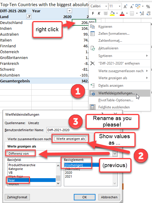
I enclose a screenshot to show you how I can show the sales increase in the 2021 sales column.
The trouble is - and you and I are not to blame for this - the bug still exists.
It looks as if the top-ten filter does not work correctly on pivot table values that have been created with the 'show value as'-functionality.
Again, thank you very much for doing such an in-depth approach.
If you still need more advice on this feature, let me know.
Thank you Bob.
thank you very much for your great efforts.
The calculated fields in my table are of no use for my goal to show the sales increase/decrease in 2021 from 2020.
Therefore they are unchecked and have no effect on my pivot table whatsoever. And you stated that at the end of your comments as well.
I enclose a screenshot to show you how I can show the sales increase in the 2021 sales column.
The trouble is - and you and I are not to blame for this - the bug still exists.
It looks as if the top-ten filter does not work correctly on pivot table values that have been created with the 'show value as'-functionality.
Again, thank you very much for doing such an in-depth approach.
If you still need more advice on this feature, let me know.
Thank you Bob.
HOLD OFF ON CALLING MICROSOFT. I AM PURSUING SOME INTERESTING THINGS ABOUT ABSOLUTE VALUES EFFECT ON TOP 10 FEATURE
Great instructions, and I am glad I learned that trick.
But I agree it looks like a bug which I have duplicated in ee2 simple proof of bug (208 records only).xlsx. It fails on two different machines under office 365 and office 2010.
Your Value Field Settings are fairly advanced. But those seem to work correctly.
The "Top 10" feature is much simpler, yet it seems to be broken.
I think it is worth reporting to Microsoft. Do you have an office 365 subscription? If so I have found theirUSA tech support is fairly good as long as you are persistent and patient, and I expect Germany's is just as good
But I have time on my hands so I would like to report the problem myself under my Office 365 subscription. (I will only send the super small file.) Please let me know if that is OK.
Of course, I don't expect a solution for several years, but they will never fix the problem if they don't know about it.
rberke (aka UncleBob).
ASKER
Hi bob, thank u very much for pursuing this thing/bug so 'rigorously', I really appreciate it.
As per your request ... HOLD OFF ON CALLING MICROSOFT. I AM PURSUING SOME INTERESTING THINGS ABOUT ABSOLUTE VALUES EFFECT ON TOP 10 FEATURE ... I will waig until further notice. Thank you Bob
As per your request ... HOLD OFF ON CALLING MICROSOFT. I AM PURSUING SOME INTERESTING THINGS ABOUT ABSOLUTE VALUES EFFECT ON TOP 10 FEATURE ... I will waig until further notice. Thank you Bob
I think I figured it out.
This is not a bug.
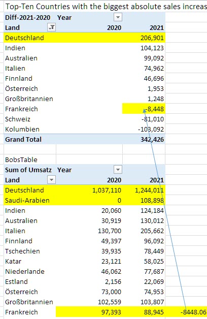
Your top 10 filter is on the whole table, not the right hand column. That can easily be seen by looking at this snip from the picture you posted earlier,
You think your top 10 filter is on a subtraction (i.e. Diff-2021-2020), but that is not what is happening.
Excel is actually using additions (i.e. Sum of Umsatz) for all years.
The text "diff-2021-2020" is an alias that you yourself chose. You could have chosen something else like "George", but it has no functional meaning.
To understand better do the following
Open the original problem workbook. https://www.experts-exchange.com/questions/29218623/Value-Filter-Top-Ten-not-working-correctly.html#
Notice the first 3 countries are Deutschland, Indien, Australien which is missing Saudi Arabia, and the Grand total is 342,486
Next change "show value as" to be "No Calculation'. This only changes the display and nothing else. (Calculations, sort sequence and filters are not affected.)
MINOR ADDITION LATER IN THE DAY: You can now use design view and turn on grand totals for columns That grand total column is being used by your Top 10 filter.
Next remove the Year from the column labels.
Your pivot now has a single unsorted dollar column with a grand total of 4,208,521. But the first 3 countries are unchanged and the grand total is just a different view of the exact same data that created 342,486.
The column heading still shows Diff-2021-2020 but it is a meaningless alias. You might want to change it back to "Sum of Umsatz"..

Now sort the pivot by the right hand column, and the top 10 still add up to to 4,208,521 but now Indien is at the bottom because it is the smallest of the 10..
Now remove the top 10 filter so you can see all the countries.
You will notice only the the top 10 were sorted by size so you must sort the right hand column an extra time to see the whole picture.
Eureka, you can see that Saudi Arabia is the 14th biggest country, and is not in the top 10.
Unfortunately, I do not know any easy way to move the top 10 filter to the right hand column. But at least we now understand what is going on.
Later this week I will look for a way to do what you want. Or maybe you can post a new question on EE.
This is not a bug.
Your top 10 filter is on the whole table, not the right hand column. That can easily be seen by looking at this snip from the picture you posted earlier,

You think your top 10 filter is on a subtraction (i.e. Diff-2021-2020), but that is not what is happening.
Excel is actually using additions (i.e. Sum of Umsatz) for all years.
The text "diff-2021-2020" is an alias that you yourself chose. You could have chosen something else like "George", but it has no functional meaning.
To understand better do the following
Open the original problem workbook. https://www.experts-exchange.com/questions/29218623/Value-Filter-Top-Ten-not-working-correctly.html#
Notice the first 3 countries are Deutschland, Indien, Australien which is missing Saudi Arabia, and the Grand total is 342,486
Next change "show value as" to be "No Calculation'. This only changes the display and nothing else. (Calculations, sort sequence and filters are not affected.)
MINOR ADDITION LATER IN THE DAY: You can now use design view and turn on grand totals for columns That grand total column is being used by your Top 10 filter.
Next remove the Year from the column labels.
Your pivot now has a single unsorted dollar column with a grand total of 4,208,521. But the first 3 countries are unchanged and the grand total is just a different view of the exact same data that created 342,486.
The column heading still shows Diff-2021-2020 but it is a meaningless alias. You might want to change it back to "Sum of Umsatz"..
Now sort the pivot by the right hand column, and the top 10 still add up to to 4,208,521 but now Indien is at the bottom because it is the smallest of the 10..
Now remove the top 10 filter so you can see all the countries.
You will notice only the the top 10 were sorted by size so you must sort the right hand column an extra time to see the whole picture.
Eureka, you can see that Saudi Arabia is the 14th biggest country, and is not in the top 10.
Unfortunately, I do not know any easy way to move the top 10 filter to the right hand column. But at least we now understand what is going on.
Later this week I will look for a way to do what you want. Or maybe you can post a new question on EE.
ASKER
Wow, great job Bob, superb work. I will go thru all the single steps one at a time to grasp everything. Again thank u very much, I highly appreciate it.
I have not found any documentation showing how to select top 10 of a specific pivot table data column, so I wrote my own.
It works fine on simple cases but it not as general as Excel's built in tools. For instance, my macro does not do Bottom 10.
Also, my macro automatically sorts the column whereas the built in leaves sort sequence unchanged. I could improve my macro to avoid this, but it would be 20% more complicated.
Also, if you ask the build in for the top 10, it may show a few more that 10 if there are "ties". I could fix that easily, but I won't bother now.
You can add it to your current .xlsm file, but it would be more useful if you put it into your personal.xls file.
You could then assign it as a hot key and use it on any your workbooks.
If you use it, keep me posted on how well it works.
Sub MyTop10()
Dim pt As Object, cnt As Long, cell As Object, Top10Value As String
' make sure user selected a valid cell

    If Selection.Cells.Count <> 1 Then
        MsgBox "To show the top 10 Select a data cell the pivot table's data area."
        Exit Sub
    End If
    For Each pt In ActiveSheet.PivotTables
        If Not Intersect(pt.DataBodyRange, Selection) Is Nothing Then
            Exit For
        End If
    Next
    If pt Is Nothing Then
        MsgBox "To show the top 10 Select a data cell the pivot table's data area."
        Exit Sub
    End If


' get users desire

    Do
        Top10Value = "xxx"
        Top10Value = InputBox("How many Top items should be shown? ", , 10)
        If Top10Value = "" Then Exit Sub  ' user canceled the input box.
    Loop Until Val(Top10Value) > 0


    ' unhide all countries before sorting, then sort them top to bottom
    Dim fld As String
    fld = "" & pt.RowRange.Cells(1)
    pt.PivotFields(fld).ClearAllFilters

    Selection.Sort Key1:=Selection, Order1:=xlDescending, Type _
            :=xlSortValues, OrderCustom:=1, Orientation:=xlTopToBottom


        For cnt = pt.RowRange.Cells.Count - 1 To Top10Value + 2 Step -1

            pt.RowRange.Cells(cnt).Delete

        Next


End Sub
ASKER
Hi Bob, wow, I am truly impressed. It works as desired.
You write: ... "Also, my macro automatically sorts the column whereas the built in leaves sort sequence unchanged. I could improve my macro to avoid this, but it would be 20% more complicated."
Comment Andreas: The automatic sorting of the value column is excactly what I want, so everything is perfekt !!
Furthermore you write: " Also, if you ask the build in for the top 10, it may show a few more that 10 if there are "ties". I could fix that easily, but I won't bother now.
Comment Andreas: What exactly do you mean by that?
Again Bob, thank you very much for your superb job. This is great!! I really highly appreciate your professional expertise.
Best Regards, Andreas
ASKER
Hi Bob, I know what you mean by ... show a few more than 10 if there are "ties". But this not relevant for my purpose/goal.
ASKER CERTIFIED SOLUTION
membership
This solution is only available to members.
To access this solution, you must be a member of Experts Exchange.
ASKER
Hi Bob,
this is great, this macro is noticeably is quicker. It works as desired. Thank you very much for going to great lengths to get this macro going perfectly. I really highly appreciate it.
Best Regards, Andreas and have a nice day.
this is great, this macro is noticeably is quicker. It works as desired. Thank you very much for going to great lengths to get this macro going perfectly. I really highly appreciate it.
Best Regards, Andreas and have a nice day.
thanks for asking the original question, I also learned a lot. And thanks for the testimonial.
Maybe close and reopen Excel.